Table of Contents
1 An example of a small Single-Player simulation
1.1 Creating the problem
1.1.1 Parameters for the simulation
1.1.2 Some MAB problem with Bernoulli arms
1.1.3 Some RL algorithms
1.2 Creating the Evaluator object
1.3 Solving the problem
1.4 Plotting the results
1.4.1 First problem
1.4.2 Second problem
1.4.3 Third problem
An example of a small Single-Player simulation
First, be sure to be in the main folder, and import Evaluator from
Environment package:
In [1]:
from sys import path
path.insert(0, '..')
In [3]:
# Local imports
from Environment import Evaluator, tqdm
We also need arms, for instance Bernoulli-distributed arm:
In [7]:
# Import arms
from Arms import Bernoulli
And finally we need some single-player Reinforcement Learning algorithms:
In [9]:
# Import algorithms
from Policies import *
For instance, this imported the `UCB
algorithm <https://en.wikipedia.org/wiki/Multi-armed_bandit#Bandit_strategies>`__
is the UCBalpha class:
In [10]:
# Just improving the ?? in Jupyter. Thanks to https://nbviewer.jupyter.org/gist/minrk/7715212
from __future__ import print_function
from IPython.core import page
def myprint(s):
    try:
        print(s['text/plain'])
    except (KeyError, TypeError):
        print(s)
page.page = myprint
In [11]:
UCBalpha?
Init signature: UCBalpha(nbArms, alpha=1, lower=0.0, amplitude=1.0)
Docstring:
The UCB1 (UCB-alpha) index policy, modified to take a random permutation order for the initial exploration of each arm (reduce collisions in the multi-players setting).
Reference: [Auer et al. 02].
Init docstring:
New generic index policy.

- nbArms: the number of arms,
- lower, amplitude: lower value and known amplitude of the rewards.
File:           ~/ownCloud/cloud.openmailbox.org/Thèse_2016-17/src/SMPyBandits.git/Policies/UCBalpha.py
Type:           type
With more details, here the code:
In [12]:
UCBalpha??
Init signature: UCBalpha(nbArms, alpha=1, lower=0.0, amplitude=1.0)
Source:
class UCBalpha(UCB):
    """ The UCB1 (UCB-alpha) index policy, modified to take a random permutation order for the initial exploration of each arm (reduce collisions in the multi-players setting).
    Reference: [Auer et al. 02].
    """

    def __init__(self, nbArms, alpha=ALPHA, lower=0., amplitude=1.):
        super(UCBalpha, self).__init__(nbArms, lower=lower, amplitude=amplitude)
        assert alpha >= 0, "Error: the alpha parameter for UCBalpha class has to be >= 0."
        self.alpha = alpha  #: Parameter alpha

    def __str__(self):
        return r"UCB($\alpha={:.3g}$)".format(self.alpha)

    def computeIndex(self, arm):
        r""" Compute the current index, at time t and after :math:`N_k(t)` pulls of arm k:

        .. math:: I_k(t) = \frac{X_k(t)}{N_k(t)} + \sqrt{\frac{\alpha \log(t)}{2 N_k(t)}}.
        """
        if self.pulls[arm] < 1:
            return float('+inf')
        else:
            return (self.rewards[arm] / self.pulls[arm]) + sqrt((self.alpha * log(self.t)) / (2 * self.pulls[arm]))

    def computeAllIndex(self):
        """ Compute the current indexes for all arms, in a vectorized manner."""
        indexes = (self.rewards / self.pulls) + np.sqrt((self.alpha * np.log(self.t)) / (2 * self.pulls))
        indexes[self.pulls < 1] = float('+inf')
        self.index = indexes
File:           ~/ownCloud/cloud.openmailbox.org/Thèse_2016-17/src/SMPyBandits.git/Policies/UCBalpha.py
Type:           type
Creating the problem
Parameters for the simulation
- \(T = 10000\) is the time horizon,
- \(N = 10\) is the number of repetitions,
N_JOBS = 4is the number of cores used to parallelize the code.
In [6]:
HORIZON = 10000
REPETITIONS = 10
N_JOBS = 4
Some MAB problem with Bernoulli arms
We consider in this example \(3\) problems, with Bernoulli arms,
of different means.
In [7]:
ENVIRONMENTS = [  # 1)  Bernoulli arms
        {   # A very easy problem, but it is used in a lot of articles
            "arm_type": Bernoulli,
            "params": [0.1, 0.2, 0.3, 0.4, 0.5, 0.6, 0.7, 0.8, 0.9]
        },
        {   # An other problem, best arm = last, with three groups: very bad arms (0.01, 0.02), middle arms (0.3 - 0.6) and very good arms (0.78, 0.8, 0.82)
            "arm_type": Bernoulli,
            "params": [0.01, 0.02, 0.3, 0.4, 0.5, 0.6, 0.795, 0.8, 0.805]
        },
        {   # A very hard problem, as used in [Cappé et al, 2012]
            "arm_type": Bernoulli,
            "params": [0.01, 0.01, 0.01, 0.02, 0.02, 0.02, 0.05, 0.05, 0.1]
        },
    ]
Some RL algorithms
We compare Thompson Sampling against \(\mathrm{UCB}_1\), and \(\mathrm{kl}-\mathrm{UCB}\).
In [8]:
POLICIES = [
        # --- UCB1 algorithm
        {
            "archtype": UCBalpha,
            "params": {
                "alpha": 1
            }
        },
        {
            "archtype": UCBalpha,
            "params": {
                "alpha": 0.5  # Smallest theoretically acceptable value
            }
        },
        # --- Thompson algorithm
        {
            "archtype": Thompson,
            "params": {}
        },
        # --- KL algorithms, here only klUCB
        {
            "archtype": klUCB,
            "params": {}
        },
        # --- BayesUCB algorithm
        {
            "archtype": BayesUCB,
            "params": {}
        },
    ]
Complete configuration for the problem:
In [9]:
configuration = {
    # --- Duration of the experiment
    "horizon": HORIZON,
    # --- Number of repetition of the experiment (to have an average)
    "repetitions": REPETITIONS,
    # --- Parameters for the use of joblib.Parallel
    "n_jobs": N_JOBS,    # = nb of CPU cores
    "verbosity": 6,      # Max joblib verbosity
    # --- Arms
    "environment": ENVIRONMENTS,
    # --- Algorithms
    "policies": POLICIES,
}
configuration
Out[9]:
{'environment': [{'arm_type': Arms.Bernoulli.Bernoulli,
   'params': [0.1, 0.2, 0.3, 0.4, 0.5, 0.6, 0.7, 0.8, 0.9]},
  {'arm_type': Arms.Bernoulli.Bernoulli,
   'params': [0.01, 0.02, 0.3, 0.4, 0.5, 0.6, 0.795, 0.8, 0.805]},
  {'arm_type': Arms.Bernoulli.Bernoulli,
   'params': [0.01, 0.01, 0.01, 0.02, 0.02, 0.02, 0.05, 0.05, 0.1]}],
 'horizon': 10000,
 'n_jobs': 4,
 'policies': [{'archtype': Policies.UCBalpha.UCBalpha, 'params': {'alpha': 1}},
  {'archtype': Policies.UCBalpha.UCBalpha, 'params': {'alpha': 0.5}},
  {'archtype': Policies.Thompson.Thompson, 'params': {}},
  {'archtype': Policies.klUCB.klUCB, 'params': {}},
  {'archtype': Policies.BayesUCB.BayesUCB, 'params': {}}],
 'repetitions': 10,
 'verbosity': 6}
Creating the Evaluator object
In [10]:
evaluation = Evaluator(configuration)
Number of policies in this comparison: 5
Time horizon: 10000
Number of repetitions: 10
Sampling rate DELTA_T_SAVE: 1
Creating a new MAB problem ...
  Reading arms of this MAB problem from a dictionnary 'configuration' = {'params': [0.1, 0.2, 0.3, 0.4, 0.5, 0.6, 0.7, 0.8, 0.9], 'arm_type': <class 'Arms.Bernoulli.Bernoulli'>} ...
 - with 'arm_type' = <class 'Arms.Bernoulli.Bernoulli'>
 - with 'params' = [0.1, 0.2, 0.3, 0.4, 0.5, 0.6, 0.7, 0.8, 0.9]
 - with 'arms' = [B(0.1), B(0.2), B(0.3), B(0.4), B(0.5), B(0.6), B(0.7), B(0.8), B(0.9)]
 - with 'nbArms' = 9
 - with 'maxArm' = 0.9
 - with 'minArm' = 0.1

This MAB problem has:
 - a [Lai & Robbins] complexity constant C(mu) = 7.52 ...
 - a Optimal Arm Identification factor H_OI(mu) = 48.89% ...
Creating a new MAB problem ...
  Reading arms of this MAB problem from a dictionnary 'configuration' = {'params': [0.01, 0.02, 0.3, 0.4, 0.5, 0.6, 0.795, 0.8, 0.805], 'arm_type': <class 'Arms.Bernoulli.Bernoulli'>} ...
 - with 'arm_type' = <class 'Arms.Bernoulli.Bernoulli'>
 - with 'params' = [0.01, 0.02, 0.3, 0.4, 0.5, 0.6, 0.795, 0.8, 0.805]
 - with 'arms' = [B(0.01), B(0.02), B(0.3), B(0.4), B(0.5), B(0.6), B(0.795), B(0.8), B(0.805)]
 - with 'nbArms' = 9
 - with 'maxArm' = 0.805
 - with 'minArm' = 0.01

This MAB problem has:
 - a [Lai & Robbins] complexity constant C(mu) = 101 ...
 - a Optimal Arm Identification factor H_OI(mu) = 55.39% ...
Creating a new MAB problem ...
  Reading arms of this MAB problem from a dictionnary 'configuration' = {'params': [0.01, 0.01, 0.01, 0.02, 0.02, 0.02, 0.05, 0.05, 0.1], 'arm_type': <class 'Arms.Bernoulli.Bernoulli'>} ...
 - with 'arm_type' = <class 'Arms.Bernoulli.Bernoulli'>
 - with 'params' = [0.01, 0.01, 0.01, 0.02, 0.02, 0.02, 0.05, 0.05, 0.1]
 - with 'arms' = [B(0.01), B(0.01), B(0.01), B(0.02), B(0.02), B(0.02), B(0.05), B(0.05), B(0.1)]
 - with 'nbArms' = 9
 - with 'maxArm' = 0.1
 - with 'minArm' = 0.01

This MAB problem has:
 - a [Lai & Robbins] complexity constant C(mu) = 14.5 ...
 - a Optimal Arm Identification factor H_OI(mu) = 82.11% ...
Number of environments to try: 3
Solving the problem
Now we can simulate all the \(3\) environments. That part can take some time.
In [16]:
for envId, env in tqdm(enumerate(evaluation.envs), desc="Problems"):
    # Evaluate just that env
    evaluation.startOneEnv(envId, env)
Evaluating environment: <MAB{'nbArms': 9, 'minArm': 0.10000000000000001, 'maxArm': 0.90000000000000002, 'arms': [B(0.1), B(0.2), B(0.3), B(0.4), B(0.5), B(0.6), B(0.7), B(0.8), B(0.9)]}>
- Adding policy #1 = {'params': {'alpha': 1}, 'archtype': <class 'Policies.UCBalpha.UCBalpha'>} ...
  Creating this policy from a dictionnary 'self.cfg['policies'][0]' = {'params': {'alpha': 1}, 'archtype': <class 'Policies.UCBalpha.UCBalpha'>} ...
- Adding policy #2 = {'params': {'alpha': 0.5}, 'archtype': <class 'Policies.UCBalpha.UCBalpha'>} ...
  Creating this policy from a dictionnary 'self.cfg['policies'][1]' = {'params': {'alpha': 0.5}, 'archtype': <class 'Policies.UCBalpha.UCBalpha'>} ...
- Adding policy #3 = {'params': {}, 'archtype': <class 'Policies.Thompson.Thompson'>} ...
  Creating this policy from a dictionnary 'self.cfg['policies'][2]' = {'params': {}, 'archtype': <class 'Policies.Thompson.Thompson'>} ...
- Adding policy #4 = {'params': {}, 'archtype': <class 'Policies.klUCB.klUCB'>} ...
  Creating this policy from a dictionnary 'self.cfg['policies'][3]' = {'params': {}, 'archtype': <class 'Policies.klUCB.klUCB'>} ...
- Adding policy #5 = {'params': {}, 'archtype': <class 'Policies.BayesUCB.BayesUCB'>} ...
  Creating this policy from a dictionnary 'self.cfg['policies'][4]' = {'params': {}, 'archtype': <class 'Policies.BayesUCB.BayesUCB'>} ...

- Evaluating policy #1/5: UCB($\alpha=1$) ...

Estimated order by the policy UCB($\alpha=1$) after 10000 steps: [0 1 2 3 4 6 5 7 8] ...  ==> Manhattan   distance from optimal ordering: 95.06% (relative success)...

  ==> Optimal arm identification: 100.00% (relative success)...
  ==> Kendell Tau distance from optimal ordering: 99.96% (relative success)...
  ==> Spearman    distance from optimal ordering: 100.00% (relative success)...
  ==> Gestalt     distance from optimal ordering: 88.89% (relative success)...
  ==> Mean distance from optimal ordering: 95.98% (relative success)...
[Parallel(n_jobs=4)]: Done   5 out of  10 | elapsed:    1.9s remaining:    1.9s
[Parallel(n_jobs=4)]: Done   7 out of  10 | elapsed:    2.1s remaining:    0.9s
[Parallel(n_jobs=4)]: Done  10 out of  10 | elapsed:    2.6s finished
- Evaluating policy #2/5: UCB($\alpha=0.5$) ...

Estimated order by the policy UCB($\alpha=0.5$) after 10000 steps: [0 1 3 2 5 4 6 7 8] ...
  ==> Optimal arm identification: 100.00% (relative success)...
  ==> Manhattan   distance from optimal ordering: 90.12% (relative success)...
  ==> Kendell Tau distance from optimal ordering: 99.92% (relative success)...
  ==> Spearman    distance from optimal ordering: 100.00% (relative success)...
  ==> Gestalt     distance from optimal ordering: 77.78% (relative success)...
  ==> Mean distance from optimal ordering: 91.95% (relative success)...
[Parallel(n_jobs=4)]: Done   5 out of  10 | elapsed:    1.9s remaining:    1.9s
[Parallel(n_jobs=4)]: Done   7 out of  10 | elapsed:    2.0s remaining:    0.9s
[Parallel(n_jobs=4)]: Done  10 out of  10 | elapsed:    2.7s finished
- Evaluating policy #3/5: Thompson ...

Estimated order by the policy Thompson after 10000 steps: [1 3 0 4 2 6 5 7 8] ...
  ==> Optimal arm identification: 100.00% (relative success)...
  ==> Manhattan   distance from optimal ordering: 75.31% (relative success)...
  ==> Kendell Tau distance from optimal ordering: 99.33% (relative success)...
  ==> Spearman    distance from optimal ordering: 99.75% (relative success)...
  ==> Gestalt     distance from optimal ordering: 66.67% (relative success)...
  ==> Mean distance from optimal ordering: 85.26% (relative success)...
[Parallel(n_jobs=4)]: Done   5 out of  10 | elapsed:    1.2s remaining:    1.2s
[Parallel(n_jobs=4)]: Done   7 out of  10 | elapsed:    1.3s remaining:    0.6s
[Parallel(n_jobs=4)]: Done  10 out of  10 | elapsed:    1.7s finished
- Evaluating policy #4/5: KL-UCB(Bern) ...

Estimated order by the policy KL-UCB(Bern) after 10000 steps: [2 3 6 0 1 5 4 7 8] ...
  ==> Optimal arm identification: 100.00% (relative success)...
  ==> Manhattan   distance from optimal ordering: 60.49% (relative success)...
  ==> Kendell Tau distance from optimal ordering: 93.94% (relative success)...
  ==> Spearman    distance from optimal ordering: 92.31% (relative success)...
  ==> Gestalt     distance from optimal ordering: 55.56% (relative success)...
  ==> Mean distance from optimal ordering: 75.57% (relative success)...
[Parallel(n_jobs=4)]: Done   5 out of  10 | elapsed:    2.1s remaining:    2.1s
[Parallel(n_jobs=4)]: Done   7 out of  10 | elapsed:    2.3s remaining:    1.0s
- Evaluating policy #5/5: BayesUCB ...
[Parallel(n_jobs=4)]: Done 10 out of 10 | elapsed: 3.1s finished
Estimated order by the policy BayesUCB after 10000 steps: [7 5 6 0 3 2 1 4 8] ...
  ==> Optimal arm identification: 100.00% (relative success)...
  ==> Manhattan   distance from optimal ordering: 25.93% (relative success)...
  ==> Kendell Tau distance from optimal ordering: 32.33% (relative success)...
  ==> Spearman    distance from optimal ordering: 23.50% (relative success)...
  ==> Gestalt     distance from optimal ordering: 33.33% (relative success)...
  ==> Mean distance from optimal ordering: 28.77% (relative success)...
[Parallel(n_jobs=4)]: Done   5 out of  10 | elapsed:    2.5s remaining:    2.5s
[Parallel(n_jobs=4)]: Done   7 out of  10 | elapsed:    2.6s remaining:    1.1s
[Parallel(n_jobs=4)]: Done  10 out of  10 | elapsed:    3.4s finished
Evaluating environment: <MAB{'nbArms': 9, 'minArm': 0.01, 'maxArm': 0.80500000000000005, 'arms': [B(0.01), B(0.02), B(0.3), B(0.4), B(0.5), B(0.6), B(0.795), B(0.8), B(0.805)]}>
- Adding policy #1 = {'params': {'alpha': 1}, 'archtype': <class 'Policies.UCBalpha.UCBalpha'>} ...
  Creating this policy from a dictionnary 'self.cfg['policies'][0]' = {'params': {'alpha': 1}, 'archtype': <class 'Policies.UCBalpha.UCBalpha'>} ...
- Adding policy #2 = {'params': {'alpha': 0.5}, 'archtype': <class 'Policies.UCBalpha.UCBalpha'>} ...
  Creating this policy from a dictionnary 'self.cfg['policies'][1]' = {'params': {'alpha': 0.5}, 'archtype': <class 'Policies.UCBalpha.UCBalpha'>} ...
- Adding policy #3 = {'params': {}, 'archtype': <class 'Policies.Thompson.Thompson'>} ...
  Creating this policy from a dictionnary 'self.cfg['policies'][2]' = {'params': {}, 'archtype': <class 'Policies.Thompson.Thompson'>} ...
- Adding policy #4 = {'params': {}, 'archtype': <class 'Policies.klUCB.klUCB'>} ...
  Creating this policy from a dictionnary 'self.cfg['policies'][3]' = {'params': {}, 'archtype': <class 'Policies.klUCB.klUCB'>} ...
- Adding policy #5 = {'params': {}, 'archtype': <class 'Policies.BayesUCB.BayesUCB'>} ...
  Creating this policy from a dictionnary 'self.cfg['policies'][4]' = {'params': {}, 'archtype': <class 'Policies.BayesUCB.BayesUCB'>} ...

- Evaluating policy #1/5: UCB($\alpha=1$) ...

Estimated order by the policy UCB($\alpha=1$) after 10000 steps: [0 1 4 2 5 3 7 8 6] ...
  ==> Optimal arm identification: 98.76% (relative success)...
  ==> Manhattan   distance from optimal ordering: 75.31% (relative success)...
  ==> Kendell Tau distance from optimal ordering: 99.33% (relative success)...
  ==> Spearman    distance from optimal ordering: 99.75% (relative success)...
  ==> Gestalt     distance from optimal ordering: 66.67% (relative success)...
  ==> Mean distance from optimal ordering: 85.26% (relative success)...
[Parallel(n_jobs=4)]: Done   5 out of  10 | elapsed:    2.1s remaining:    2.1s
[Parallel(n_jobs=4)]: Done   7 out of  10 | elapsed:    2.2s remaining:    0.9s
- Evaluating policy #2/5: UCB($\alpha=0.5$) ...
[Parallel(n_jobs=4)]: Done 10 out of 10 | elapsed: 2.8s finished
Estimated order by the policy UCB($\alpha=0.5$) after 10000 steps: [0 1 2 3 4 5 8 6 7] ...
  ==> Optimal arm identification: 99.38% (relative success)...
  ==> Manhattan   distance from optimal ordering: 90.12% (relative success)...
  ==> Kendell Tau distance from optimal ordering: 99.92% (relative success)...
  ==> Spearman    distance from optimal ordering: 99.99% (relative success)...
  ==> Gestalt     distance from optimal ordering: 88.89% (relative success)...
  ==> Mean distance from optimal ordering: 94.73% (relative success)...
[Parallel(n_jobs=4)]: Done   5 out of  10 | elapsed:    1.9s remaining:    1.9s
[Parallel(n_jobs=4)]: Done   7 out of  10 | elapsed:    2.0s remaining:    0.9s
- Evaluating policy #3/5: Thompson ...
[Parallel(n_jobs=4)]: Done 10 out of 10 | elapsed: 2.6s finished
Estimated order by the policy Thompson after 10000 steps: [0 5 1 2 3 4 7 8 6] ...
  ==> Optimal arm identification: 98.76% (relative success)...
  ==> Manhattan   distance from optimal ordering: 70.37% (relative success)...
  ==> Kendell Tau distance from optimal ordering: 98.77% (relative success)...
  ==> Spearman    distance from optimal ordering: 98.75% (relative success)...
  ==> Gestalt     distance from optimal ordering: 77.78% (relative success)...
  ==> Mean distance from optimal ordering: 86.42% (relative success)...
[Parallel(n_jobs=4)]: Done   5 out of  10 | elapsed:    1.2s remaining:    1.2s
[Parallel(n_jobs=4)]: Done   7 out of  10 | elapsed:    1.3s remaining:    0.5s
[Parallel(n_jobs=4)]: Done  10 out of  10 | elapsed:    1.6s finished
- Evaluating policy #4/5: KL-UCB(Bern) ...

Estimated order by the policy KL-UCB(Bern) after 10000 steps: [0 1 3 4 2 5 8 6 7] ...
  ==> Optimal arm identification: 99.38% (relative success)...
  ==> Manhattan   distance from optimal ordering: 80.25% (relative success)...
  ==> Kendell Tau distance from optimal ordering: 99.65% (relative success)...
  ==> Spearman    distance from optimal ordering: 99.91% (relative success)...
  ==> Gestalt     distance from optimal ordering: 77.78% (relative success)...
  ==> Mean distance from optimal ordering: 89.39% (relative success)...
[Parallel(n_jobs=4)]: Done   5 out of  10 | elapsed:    2.2s remaining:    2.2s
[Parallel(n_jobs=4)]: Done   7 out of  10 | elapsed:    2.3s remaining:    1.0s
- Evaluating policy #5/5: BayesUCB ...
[Parallel(n_jobs=4)]: Done 10 out of 10 | elapsed: 2.9s finished
Estimated order by the policy BayesUCB after 10000 steps: [0 1 2 3 5 4 7 6 8] ...
  ==> Optimal arm identification: 100.00% (relative success)...
  ==> Manhattan   distance from optimal ordering: 90.12% (relative success)...
  ==> Kendell Tau distance from optimal ordering: 99.92% (relative success)...
  ==> Spearman    distance from optimal ordering: 100.00% (relative success)...
  ==> Gestalt     distance from optimal ordering: 77.78% (relative success)...
  ==> Mean distance from optimal ordering: 91.95% (relative success)...
[Parallel(n_jobs=4)]: Done   5 out of  10 | elapsed:    2.6s remaining:    2.6s
[Parallel(n_jobs=4)]: Done   7 out of  10 | elapsed:    2.7s remaining:    1.1s
Evaluating environment: <MAB{'nbArms': 9, 'minArm': 0.01, 'maxArm': 0.10000000000000001, 'arms': [B(0.01), B(0.01), B(0.01), B(0.02), B(0.02), B(0.02), B(0.05), B(0.05), B(0.1)]}>
- Adding policy #1 = {'params': {'alpha': 1}, 'archtype': <class 'Policies.UCBalpha.UCBalpha'>} ...
  Creating this policy from a dictionnary 'self.cfg['policies'][0]' = {'params': {'alpha': 1}, 'archtype': <class 'Policies.UCBalpha.UCBalpha'>} ...
- Adding policy #2 = {'params': {'alpha': 0.5}, 'archtype': <class 'Policies.UCBalpha.UCBalpha'>} ...
  Creating this policy from a dictionnary 'self.cfg['policies'][1]' = {'params': {'alpha': 0.5}, 'archtype': <class 'Policies.UCBalpha.UCBalpha'>} ...
- Adding policy #3 = {'params': {}, 'archtype': <class 'Policies.Thompson.Thompson'>} ...
  Creating this policy from a dictionnary 'self.cfg['policies'][2]' = {'params': {}, 'archtype': <class 'Policies.Thompson.Thompson'>} ...
- Adding policy #4 = {'params': {}, 'archtype': <class 'Policies.klUCB.klUCB'>} ...
  Creating this policy from a dictionnary 'self.cfg['policies'][3]' = {'params': {}, 'archtype': <class 'Policies.klUCB.klUCB'>} ...
- Adding policy #5 = {'params': {}, 'archtype': <class 'Policies.BayesUCB.BayesUCB'>} ...
  Creating this policy from a dictionnary 'self.cfg['policies'][4]' = {'params': {}, 'archtype': <class 'Policies.BayesUCB.BayesUCB'>} ...

- Evaluating policy #1/5: UCB($\alpha=1$) ...
[Parallel(n_jobs=4)]: Done 10 out of 10 | elapsed: 3.5s finished
Estimated order by the policy UCB($\alpha=1$) after 10000 steps: [0 1 4 5 3 7 6 2 8] ...
  ==> Optimal arm identification: 100.00% (relative success)...
  ==> Manhattan   distance from optimal ordering: 70.37% (relative success)...
  ==> Kendell Tau distance from optimal ordering: 96.29% (relative success)...
  ==> Spearman    distance from optimal ordering: 95.76% (relative success)...
  ==> Gestalt     distance from optimal ordering: 66.67% (relative success)...
  ==> Mean distance from optimal ordering: 82.27% (relative success)...
[Parallel(n_jobs=4)]: Done   5 out of  10 | elapsed:    2.0s remaining:    2.0s
[Parallel(n_jobs=4)]: Done   7 out of  10 | elapsed:    2.1s remaining:    0.9s
- Evaluating policy #2/5: UCB($\alpha=0.5$) ...
[Parallel(n_jobs=4)]: Done 10 out of 10 | elapsed: 2.8s finished
Estimated order by the policy UCB($\alpha=0.5$) after 10000 steps: [3 0 1 2 4 5 7 6 8] ...
  ==> Optimal arm identification: 100.00% (relative success)...
  ==> Manhattan   distance from optimal ordering: 80.25% (relative success)...
  ==> Kendell Tau distance from optimal ordering: 99.65% (relative success)...
  ==> Spearman    distance from optimal ordering: 99.84% (relative success)...
  ==> Gestalt     distance from optimal ordering: 77.78% (relative success)...
  ==> Mean distance from optimal ordering: 89.38% (relative success)...
[Parallel(n_jobs=4)]: Done   5 out of  10 | elapsed:    2.0s remaining:    2.0s
[Parallel(n_jobs=4)]: Done   7 out of  10 | elapsed:    2.0s remaining:    0.9s
- Evaluating policy #3/5: Thompson ...
[Parallel(n_jobs=4)]: Done 10 out of 10 | elapsed: 2.6s finished
Estimated order by the policy Thompson after 10000 steps: [3 5 2 6 4 1 0 7 8] ...
  ==> Optimal arm identification: 100.00% (relative success)...
  ==> Manhattan   distance from optimal ordering: 50.62% (relative success)...
  ==> Kendell Tau distance from optimal ordering: 46.84% (relative success)...
  ==> Spearman    distance from optimal ordering: 54.00% (relative success)...
  ==> Gestalt     distance from optimal ordering: 55.56% (relative success)...
  ==> Mean distance from optimal ordering: 51.75% (relative success)...
[Parallel(n_jobs=4)]: Done   5 out of  10 | elapsed:    1.1s remaining:    1.1s
[Parallel(n_jobs=4)]: Done   7 out of  10 | elapsed:    1.3s remaining:    0.6s
[Parallel(n_jobs=4)]: Done  10 out of  10 | elapsed:    1.6s finished
- Evaluating policy #4/5: KL-UCB(Bern) ...

Estimated order by the policy KL-UCB(Bern) after 10000 steps: [0 6 2 3 1 7 4 5 8] ...
  ==> Optimal arm identification: 100.00% (relative success)...
  ==> Manhattan   distance from optimal ordering: 65.43% (relative success)...
  ==> Kendell Tau distance from optimal ordering: 93.94% (relative success)...
  ==> Spearman    distance from optimal ordering: 92.31% (relative success)...
  ==> Gestalt     distance from optimal ordering: 66.67% (relative success)...
  ==> Mean distance from optimal ordering: 79.59% (relative success)...
[Parallel(n_jobs=4)]: Done   5 out of  10 | elapsed:    2.2s remaining:    2.2s
[Parallel(n_jobs=4)]: Done   7 out of  10 | elapsed:    2.4s remaining:    1.0s
- Evaluating policy #5/5: BayesUCB ...
[Parallel(n_jobs=4)]: Done 10 out of 10 | elapsed: 3.5s finished
Estimated order by the policy BayesUCB after 10000 steps: [0 1 5 6 4 7 2 3 8] ...
  ==> Optimal arm identification: 100.00% (relative success)...
  ==> Manhattan   distance from optimal ordering: 60.49% (relative success)...
  ==> Kendell Tau distance from optimal ordering: 90.47% (relative success)...
  ==> Spearman    distance from optimal ordering: 87.50% (relative success)...
  ==> Gestalt     distance from optimal ordering: 66.67% (relative success)...
  ==> Mean distance from optimal ordering: 76.28% (relative success)...
[Parallel(n_jobs=4)]: Done   5 out of  10 | elapsed:    4.3s remaining:    4.3s
[Parallel(n_jobs=4)]: Done   7 out of  10 | elapsed:    5.0s remaining:    2.1s
[Parallel(n_jobs=4)]: Done 10 out of 10 | elapsed: 6.4s finished
Plotting the results
And finally, visualize them, with the plotting method of a Evaluator
object:
In [12]:
def plotAll(evaluation, envId):
    evaluation.printFinalRanking(envId)
    evaluation.plotRegrets(envId)
    evaluation.plotRegrets(envId, semilogx=True)
    evaluation.plotRegrets(envId, meanRegret=True)
    evaluation.plotBestArmPulls(envId)
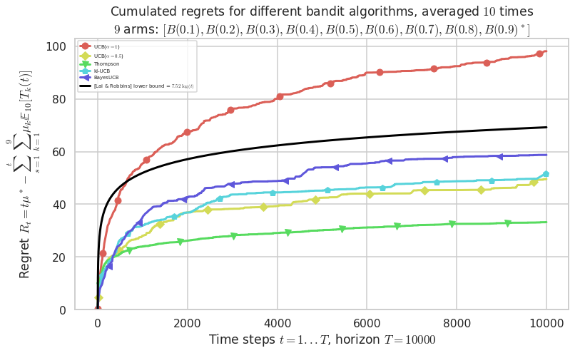
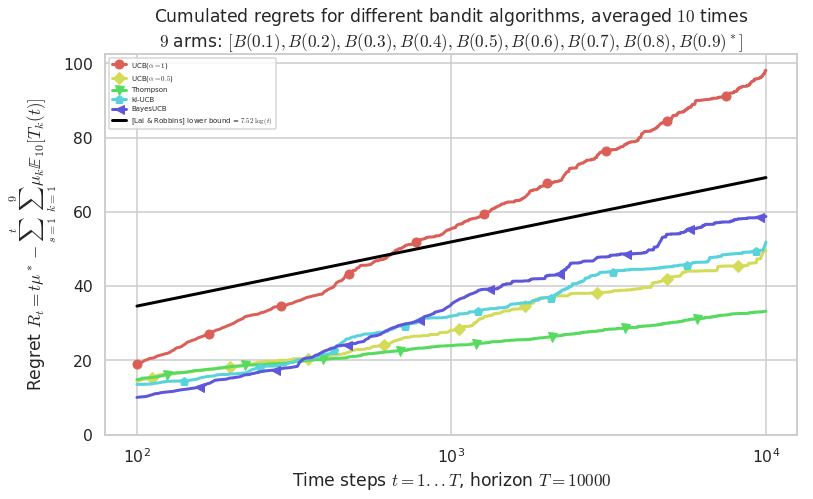
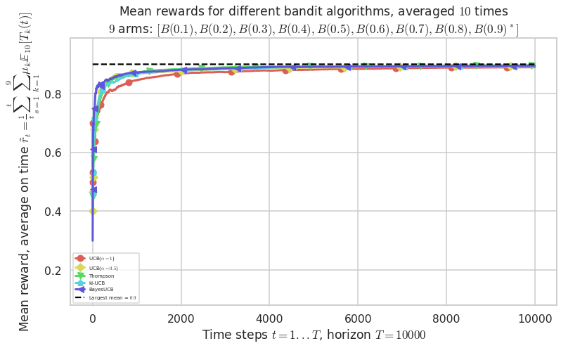
First problem
\([B(0.1), B(0.2), B(0.3), B(0.4), B(0.5), B(0.6), B(0.7), B(0.8), B(0.9)]\)
In [13]:
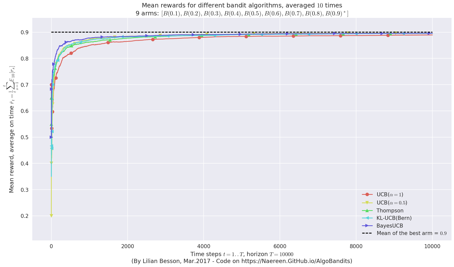
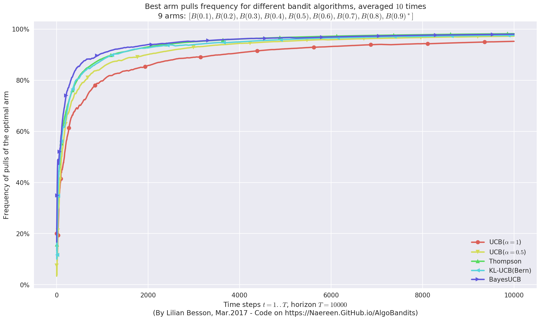
plotAll(evaluation, 0)
Final ranking for this environment #0 :
- Policy 'BayesUCB'     was ranked      1 / 5 for this simulation (last regret = 41.8).
- Policy 'UCB($\alpha=0.5$)'    was ranked      2 / 5 for this simulation (last regret = 41.9).
- Policy 'Thompson'     was ranked      3 / 5 for this simulation (last regret = 47.8).
- Policy 'KL-UCB(Bern)' was ranked      4 / 5 for this simulation (last regret = 48.7).
- Policy 'UCB($\alpha=1$)'      was ranked      5 / 5 for this simulation (last regret = 105.7).

This MAB problem has:
 - a [Lai & Robbins] complexity constant C(mu) = 7.52 for 1-player problem...
 - a Optimal Arm Identification factor H_OI(mu) = 48.89% ...
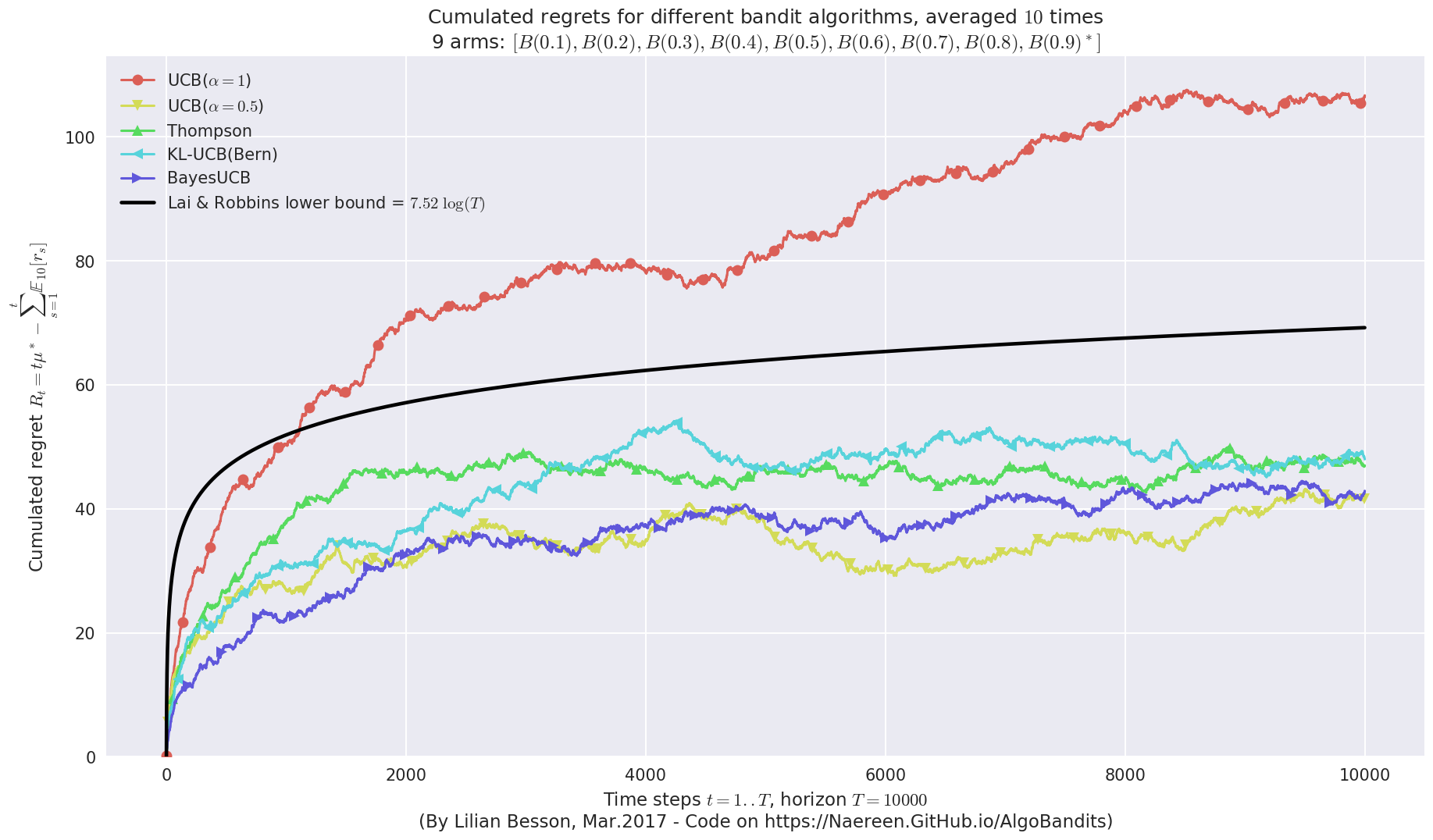
This MAB problem has:
 - a [Lai & Robbins] complexity constant C(mu) = 7.52 for 1-player problem...
 - a Optimal Arm Identification factor H_OI(mu) = 48.89% ...
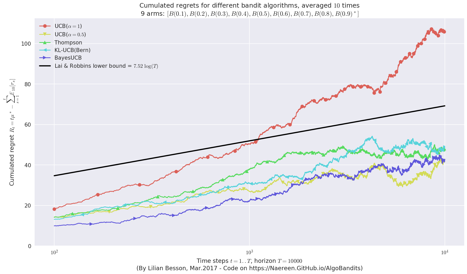
This MAB problem has:
 - a [Lai & Robbins] complexity constant C(mu) = 7.52 for 1-player problem...
 - a Optimal Arm Identification factor H_OI(mu) = 48.89% ...
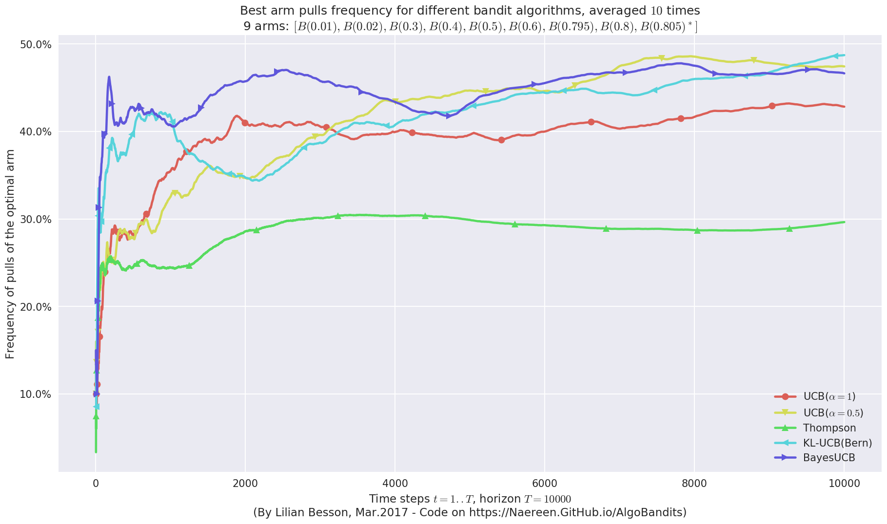
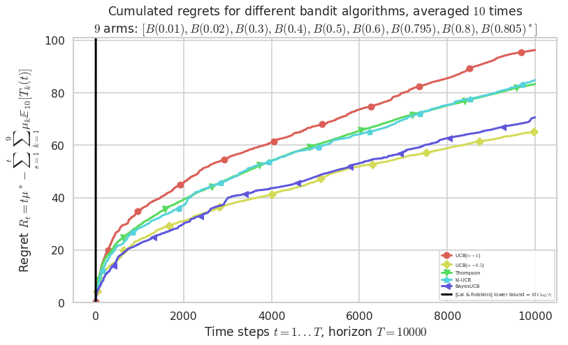
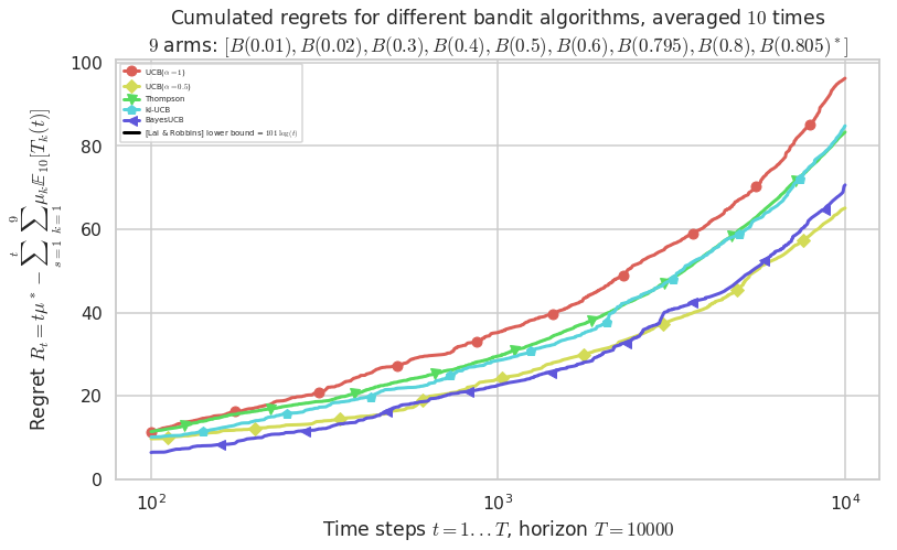
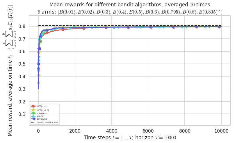
Second problem
\([B(0.01), B(0.02), B(0.3), B(0.4), B(0.5), B(0.6), B(0.795), B(0.8), B(0.805)]\)
In [14]:
plotAll(evaluation, 1)
Final ranking for this environment #1 :
- Policy 'UCB($\alpha=0.5$)'    was ranked      1 / 5 for this simulation (last regret = 65.155).
- Policy 'BayesUCB'     was ranked      2 / 5 for this simulation (last regret = 81.655).
- Policy 'Thompson'     was ranked      3 / 5 for this simulation (last regret = 84.555).
- Policy 'UCB($\alpha=1$)'      was ranked      4 / 5 for this simulation (last regret = 87.455).
- Policy 'KL-UCB(Bern)' was ranked      5 / 5 for this simulation (last regret = 88.655).

This MAB problem has:
 - a [Lai & Robbins] complexity constant C(mu) = 101 for 1-player problem...
 - a Optimal Arm Identification factor H_OI(mu) = 55.39% ...
This MAB problem has:
 - a [Lai & Robbins] complexity constant C(mu) = 101 for 1-player problem...
 - a Optimal Arm Identification factor H_OI(mu) = 55.39% ...
This MAB problem has:
 - a [Lai & Robbins] complexity constant C(mu) = 101 for 1-player problem...
 - a Optimal Arm Identification factor H_OI(mu) = 55.39% ...
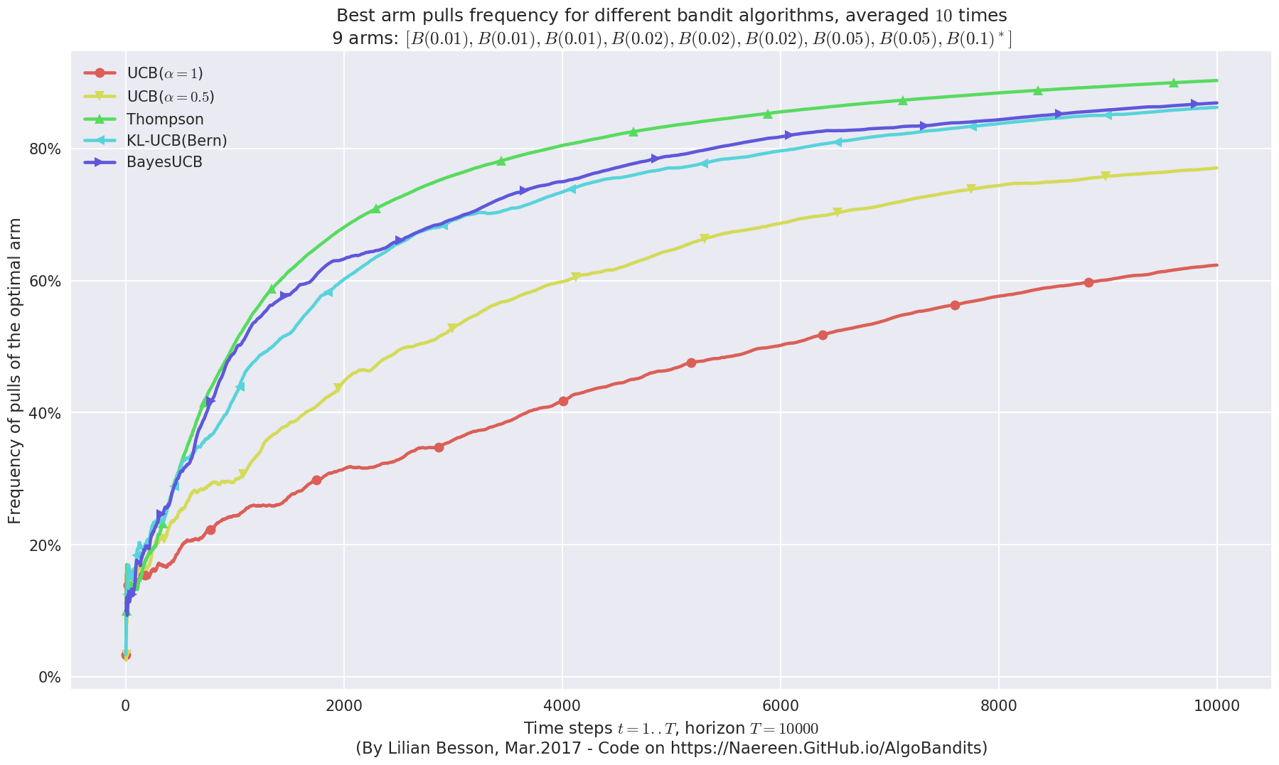
Third problem
\([B(0.01), B(0.01), B(0.01), B(0.02), B(0.02), B(0.02), B(0.05), B(0.05), B(0.1)]\)
In [15]:
plotAll(evaluation, 2)
Final ranking for this environment #2 :
- Policy 'Thompson'     was ranked      1 / 5 for this simulation (last regret = 60.4).
- Policy 'BayesUCB'     was ranked      2 / 5 for this simulation (last regret = 82.9).
- Policy 'KL-UCB(Bern)' was ranked      3 / 5 for this simulation (last regret = 92.1).
- Policy 'UCB($\alpha=0.5$)'    was ranked      4 / 5 for this simulation (last regret = 144.1).
- Policy 'UCB($\alpha=1$)'      was ranked      5 / 5 for this simulation (last regret = 253.7).

This MAB problem has:
 - a [Lai & Robbins] complexity constant C(mu) = 14.5 for 1-player problem...
 - a Optimal Arm Identification factor H_OI(mu) = 82.11% ...
This MAB problem has:
 - a [Lai & Robbins] complexity constant C(mu) = 14.5 for 1-player problem...
 - a Optimal Arm Identification factor H_OI(mu) = 82.11% ...
This MAB problem has:
 - a [Lai & Robbins] complexity constant C(mu) = 14.5 for 1-player problem...
 - a Optimal Arm Identification factor H_OI(mu) = 82.11% ...
That’s it for this demo!