Table of Contents
1 Do we even need a smart learning algorithm? Is UCB useless?
1.1 Notations for the arms
1.2 Importing the algorithms
1.3 The UCB algorithm
1.4 The EmpiricalMeans algorithm
1.5 Creating some MAB problems
1.5.1 Parameters for the simulation
1.5.2 Some MAB problem with Bernoulli arms
1.5.3 Some RL algorithms
1.6 Creating the Evaluator object
1.7 Solving the problem
1.8 Plotting the results
1.8.1 First problem
1.8.2 Second problem
1.8.3 Third problem
1.9 Conclusion
Do we even need a smart learning algorithm? Is UCB useless?
This short notebook demonstrates that “smart” Multi-Armed Bandits learning algorithms, like UCB, are indeed needed to learn the distribution of arms, even in the simplest case.
We will use an example of a small Single-Player simulation, and compare the UCB algorithm with a naive “max empirical reward” algorithm. The goal is to illustrate that introducing an exploration term (the confidence width), like what is done in UCB and similar algorithms, really helps learning and improves performance.
Notations for the arms
To remind the usual notations, there is a fixed number \(K \geq 1\) of levers, or “arms”, and a player has to select one lever at each discrete times \(t \geq 1, t \in \mathbb{N}\), ie \(k = A(t)\). Selecting an arm \(k\) at time \(t\) will yield a (random) reward, \(r_k(t)\), and the goal of the player is to maximize its cumulative reward \(R_T = \sum_{t = 1}^T r_{A(t)}(t)\).
Each arm is associated with a distribution \(\nu_k\), for \(k = 1,\dots,K\), and the usual restriction is to consider one-dimensional exponential family (it includes Gaussian, Exponential and Bernoulli distributions), ie distributions parametered by their means, \(\mu_k\). So the arm \(k\), \(r_k(t) \sim \nu_k\), are iid, and assumed bounded in \([a,b] = [0,1]\).
For instance, arms can follow Bernoulli distributions, of means \(\mu_1,\dots,\mu_K \in [0,1]\): \(r_k(t) \sim \mathrm{Bern}(\mu_k)\), ie \(\mathbb{P}(r_k(t) = 1) = \mu_k\).
Let \(N_k(t) = \sum_{\tau=1}^t \mathbb{1}(A(t) = k)\) be the number of times arm \(k\) was selected up-to time \(t \geq 1\). The empirical mean of arm \(k\) is then defined as \(\hat{\mu_k}(t) := \frac{\sum_{\tau=1}^t \mathbb{1}(A(t) = k) r_k(t) }{N_k(t)}\).
Importing the algorithms
First, be sure to be in the main folder, and import Evaluator from Environment package:
[1]:
# Local imports
from SMPyBandits.Environment import Evaluator, tqdm
Info: Using the Jupyter notebook version of the tqdm() decorator, tqdm_notebook() ...
We also need arms, for instance Bernoulli-distributed arm:
[2]:
# Import arms
from SMPyBandits.Arms import Bernoulli
And finally we need some single-player Reinforcement Learning algorithms. I focus here on the UCB index policy, and the base class IndexPolicy will be used to easily define another algorithm.
[3]:
# Import algorithms
from SMPyBandits.Policies import UCB, UCBalpha, EmpiricalMeans
from SMPyBandits.Policies.IndexPolicy import IndexPolicy
The UCB algorithm
First, we can check the documentation of the UCB class, implementing the Upper-Confidence Bounds algorithm.
[4]:
# Just improving the ?? in Jupyter. Thanks to https://nbviewer.jupyter.org/gist/minrk/7715212
from __future__ import print_function
from IPython.core import page
def myprint(s):
    try:
        print(s['text/plain'])
    except (KeyError, TypeError):
        print(s)
page.page = myprint
[5]:
UCB?
Init signature: UCB(nbArms, lower=0.0, amplitude=1.0)
Docstring:
The UCB policy for bounded bandits.

- Reference: [Lai & Robbins, 1985].
Init docstring:
New generic index policy.

- nbArms: the number of arms,
- lower, amplitude: lower value and known amplitude of the rewards.
File:           /tmp/SMPyBandits/notebooks/venv3/lib/python3.6/site-packages/SMPyBandits/Policies/UCB.py
Type:           type
Let us quickly have a look to the code of the UCB policy imported above.
[6]:
UCB??
Init signature: UCB(nbArms, lower=0.0, amplitude=1.0)
Source:
class UCB(IndexPolicy):
    """ The UCB policy for bounded bandits.

    - Reference: [Lai & Robbins, 1985].
    """

    def computeIndex(self, arm):
        r""" Compute the current index, at time t and after :math:`N_k(t)` pulls of arm k:

        .. math:: I_k(t) = \frac{X_k(t)}{N_k(t)} + \sqrt{\frac{2 \log(t)}{N_k(t)}}.
        """
        if self.pulls[arm] < 1:
            return float('+inf')
        else:
            return (self.rewards[arm] / self.pulls[arm]) + sqrt((2 * log(self.t)) / self.pulls[arm])

    def computeAllIndex(self):
        """ Compute the current indexes for all arms, in a vectorized manner."""
        indexes = (self.rewards / self.pulls) + np.sqrt((2 * np.log(self.t)) / self.pulls)
        indexes[self.pulls < 1] = float('+inf')
        self.index[:] = indexes
File:           /tmp/SMPyBandits/notebooks/venv3/lib/python3.6/site-packages/SMPyBandits/Policies/UCB.py
Type:           type
This policy is defined by inheriting from IndexPolicy, which is a generic class already implementing all the methods (choice() to get \(A(t) \in \{1,\dots,K\}\), etc). The only method defined in this class is the computeIndex(arm) method, which here uses a UCB index: the empirical mean plus a confidence width term (hence the name “upper confidence bound”).
For the classical UCB algorithm, with \(\alpha=4\), the index is computed in two parts:
the empirical mean: \(\hat{\mu}_k(t) := \frac{\sum_{\tau=1}^t \mathbb{1}(A(t) = k) r_k(t) }{N_k(t)}\), computed as
rewards[k] / pulls[k]in the code,the upper confidence bound, \(B_k(t) := \sqrt{\frac{\alpha \log(t)}{2 N_k(t)}}\), computed as
sqrt((2 * log(t)) / pulls[k]in the code.
Then the index \(X_k(t) = \hat{\mu}_k(t) + B_k(t)\) is used to decide which arm to select at time \(t+1\):
The simple UCB1 algorithm uses \(\alpha = 4\), but empirically \(\alpha = 1\) is known to work better.
The EmpiricalMeans algorithm
We can write a new bandit algorithm quite easily with my framework. For simple index-based policy, we simply need to write a computeIndex(arm) method, as presented above.
The EmpiricalMeans algorithm will be simpler than UCB, as the decision will only be based on the empirical means \(\hat{\mu}_k(t)\):
[7]:
EmpiricalMeans?
Init signature: EmpiricalMeans(nbArms, lower=0.0, amplitude=1.0)
Docstring:      The naive Empirical Means policy for bounded bandits: like UCB but without a bias correction term. Note that it is equal to UCBalpha with alpha=0, only quicker.
Init docstring:
New generic index policy.

- nbArms: the number of arms,
- lower, amplitude: lower value and known amplitude of the rewards.
File:           /tmp/SMPyBandits/notebooks/venv3/lib/python3.6/site-packages/SMPyBandits/Policies/EmpiricalMeans.py
Type:           type
[8]:
EmpiricalMeans??
Init signature: EmpiricalMeans(nbArms, lower=0.0, amplitude=1.0)
Source:
class EmpiricalMeans(IndexPolicy):
    """ The naive Empirical Means policy for bounded bandits: like UCB but without a bias correction term. Note that it is equal to UCBalpha with alpha=0, only quicker."""

    def computeIndex(self, arm):
        r""" Compute the current index, at time t and after :math:`N_k(t)` pulls of arm k:

        .. math:: I_k(t) = \frac{X_k(t)}{N_k(t)}.
        """
        if self.pulls[arm] < 1:
            return float('+inf')
        else:
            return self.rewards[arm] / self.pulls[arm]

    def computeAllIndex(self):
        """ Compute the current indexes for all arms, in a vectorized manner."""
        indexes = self.rewards / self.pulls
        indexes[self.pulls < 1] = float('+inf')
        self.index[:] = indexes
File:           /tmp/SMPyBandits/notebooks/venv3/lib/python3.6/site-packages/SMPyBandits/Policies/EmpiricalMeans.py
Type:           type
Creating some MAB problems
Parameters for the simulation
\(T = 10000\) is the time horizon,
\(N = 100\) is the number of repetitions,
N_JOBS = 4is the number of cores used to parallelize the code.
[9]:
HORIZON = 10000
REPETITIONS = 100
N_JOBS = 4
Some MAB problem with Bernoulli arms
We consider in this example \(3\) problems, with Bernoulli arms, of different means.
[10]:
ENVIRONMENTS = [  # 1)  Bernoulli arms
        {   # A very easy problem, but it is used in a lot of articles
            "arm_type": Bernoulli,
            "params": [0.1, 0.2, 0.3, 0.4, 0.5, 0.6, 0.7, 0.8, 0.9]
        },
        {   # An other problem, best arm = last, with three groups: very bad arms (0.01, 0.02), middle arms (0.3 - 0.6) and very good arms (0.78, 0.8, 0.82)
            "arm_type": Bernoulli,
            "params": [0.01, 0.02, 0.3, 0.4, 0.5, 0.6, 0.795, 0.8, 0.805]
        },
        {   # A very hard problem, as used in [Cappé et al, 2012]
            "arm_type": Bernoulli,
            "params": [0.01, 0.01, 0.01, 0.02, 0.02, 0.02, 0.05, 0.05, 0.1]
        },
    ]
Some RL algorithms
We simply want to compare the \(\mathrm{UCB}_1\) algorithm (UCB) against the EmpiricalMeans algorithm, defined above.
[11]:
POLICIES = [
        # --- UCB1 algorithm
        {
            "archtype": UCB,
            "params": {}
        },
        # --- UCB alpha algorithm with alpha=1/2
        {
            "archtype": UCBalpha,
            "params": {
                "alpha": 0.5
            }
        },
        # --- EmpiricalMeans algorithm
        {
            "archtype": EmpiricalMeans,
            "params": {}
        },
    ]
So the complete configuration for the problem will be this dictionary:
[12]:
configuration = {
    # --- Duration of the experiment
    "horizon": HORIZON,
    # --- Number of repetition of the experiment (to have an average)
    "repetitions": REPETITIONS,
    # --- Parameters for the use of joblib.Parallel
    "n_jobs": N_JOBS,    # = nb of CPU cores
    "verbosity": 6,      # Max joblib verbosity
    # --- Arms
    "environment": ENVIRONMENTS,
    # --- Algorithms
    "policies": POLICIES,
}
configuration
[12]:
{'horizon': 10000,
 'repetitions': 100,
 'n_jobs': 4,
 'verbosity': 6,
 'environment': [{'arm_type': SMPyBandits.Arms.Bernoulli.Bernoulli,
   'params': [0.1, 0.2, 0.3, 0.4, 0.5, 0.6, 0.7, 0.8, 0.9]},
  {'arm_type': SMPyBandits.Arms.Bernoulli.Bernoulli,
   'params': [0.01, 0.02, 0.3, 0.4, 0.5, 0.6, 0.795, 0.8, 0.805]},
  {'arm_type': SMPyBandits.Arms.Bernoulli.Bernoulli,
   'params': [0.01, 0.01, 0.01, 0.02, 0.02, 0.02, 0.05, 0.05, 0.1]}],
 'policies': [{'archtype': SMPyBandits.Policies.UCB.UCB, 'params': {}},
  {'archtype': SMPyBandits.Policies.UCBalpha.UCBalpha,
   'params': {'alpha': 0.5}},
  {'archtype': SMPyBandits.Policies.EmpiricalMeans.EmpiricalMeans,
   'params': {}}]}
Creating the Evaluator object
[13]:
evaluation = Evaluator(configuration)
Number of policies in this comparison: 3
Time horizon: 10000
Number of repetitions: 100
Sampling rate for plotting, delta_t_plot: 1
Number of jobs for parallelization: 4
Using this dictionary to create a new environment:
 {'arm_type': <class 'SMPyBandits.Arms.Bernoulli.Bernoulli'>, 'params': [0.1, 0.2, 0.3, 0.4, 0.5, 0.6, 0.7, 0.8, 0.9]}


Creating a new MAB problem ...
  Reading arms of this MAB problem from a dictionnary 'configuration' = {'arm_type': <class 'SMPyBandits.Arms.Bernoulli.Bernoulli'>, 'params': [0.1, 0.2, 0.3, 0.4, 0.5, 0.6, 0.7, 0.8, 0.9]} ...
 - with 'arm_type' = <class 'SMPyBandits.Arms.Bernoulli.Bernoulli'>
 - with 'params' = [0.1, 0.2, 0.3, 0.4, 0.5, 0.6, 0.7, 0.8, 0.9]
 - with 'arms' = [B(0.1), B(0.2), B(0.3), B(0.4), B(0.5), B(0.6), B(0.7), B(0.8), B(0.9)]
 - with 'means' = [0.1 0.2 0.3 0.4 0.5 0.6 0.7 0.8 0.9]
 - with 'nbArms' = 9
 - with 'maxArm' = 0.9
 - with 'minArm' = 0.1

This MAB problem has:
 - a [Lai & Robbins] complexity constant C(mu) = 7.52 ...
 - a Optimal Arm Identification factor H_OI(mu) = 48.89% ...
 - with 'arms' represented as: $[B(0.1), B(0.2), B(0.3), B(0.4), B(0.5), B(0.6), B(0.7), B(0.8), B(0.9)^*]$
Using this dictionary to create a new environment:
 {'arm_type': <class 'SMPyBandits.Arms.Bernoulli.Bernoulli'>, 'params': [0.01, 0.02, 0.3, 0.4, 0.5, 0.6, 0.795, 0.8, 0.805]}


Creating a new MAB problem ...
  Reading arms of this MAB problem from a dictionnary 'configuration' = {'arm_type': <class 'SMPyBandits.Arms.Bernoulli.Bernoulli'>, 'params': [0.01, 0.02, 0.3, 0.4, 0.5, 0.6, 0.795, 0.8, 0.805]} ...
 - with 'arm_type' = <class 'SMPyBandits.Arms.Bernoulli.Bernoulli'>
 - with 'params' = [0.01, 0.02, 0.3, 0.4, 0.5, 0.6, 0.795, 0.8, 0.805]
 - with 'arms' = [B(0.01), B(0.02), B(0.3), B(0.4), B(0.5), B(0.6), B(0.795), B(0.8), B(0.805)]
 - with 'means' = [0.01  0.02  0.3   0.4   0.5   0.6   0.795 0.8   0.805]
 - with 'nbArms' = 9
 - with 'maxArm' = 0.805
 - with 'minArm' = 0.01

This MAB problem has:
 - a [Lai & Robbins] complexity constant C(mu) = 101 ...
 - a Optimal Arm Identification factor H_OI(mu) = 55.39% ...
 - with 'arms' represented as: $[B(0.01), B(0.02), B(0.3), B(0.4), B(0.5), B(0.6), B(0.795), B(0.8), B(0.805)^*]$
Using this dictionary to create a new environment:
 {'arm_type': <class 'SMPyBandits.Arms.Bernoulli.Bernoulli'>, 'params': [0.01, 0.01, 0.01, 0.02, 0.02, 0.02, 0.05, 0.05, 0.1]}


Creating a new MAB problem ...
  Reading arms of this MAB problem from a dictionnary 'configuration' = {'arm_type': <class 'SMPyBandits.Arms.Bernoulli.Bernoulli'>, 'params': [0.01, 0.01, 0.01, 0.02, 0.02, 0.02, 0.05, 0.05, 0.1]} ...
 - with 'arm_type' = <class 'SMPyBandits.Arms.Bernoulli.Bernoulli'>
 - with 'params' = [0.01, 0.01, 0.01, 0.02, 0.02, 0.02, 0.05, 0.05, 0.1]
 - with 'arms' = [B(0.01), B(0.01), B(0.01), B(0.02), B(0.02), B(0.02), B(0.05), B(0.05), B(0.1)]
 - with 'means' = [0.01 0.01 0.01 0.02 0.02 0.02 0.05 0.05 0.1 ]
 - with 'nbArms' = 9
 - with 'maxArm' = 0.1
 - with 'minArm' = 0.01

This MAB problem has:
 - a [Lai & Robbins] complexity constant C(mu) = 14.5 ...
 - a Optimal Arm Identification factor H_OI(mu) = 82.11% ...
 - with 'arms' represented as: $[B(0.01), B(0.01), B(0.01), B(0.02), B(0.02), B(0.02), B(0.05), B(0.05), B(0.1)^*]$
Number of environments to try: 3
Solving the problem
Now we can simulate all the \(3\) environments. That part can take some time.
[14]:
for envId, env in tqdm(enumerate(evaluation.envs), desc="Problems"):
    # Evaluate just that env
    evaluation.startOneEnv(envId, env)
Evaluating environment: MAB(nbArms: 9, arms: [B(0.1), B(0.2), B(0.3), B(0.4), B(0.5), B(0.6), B(0.7), B(0.8), B(0.9)], minArm: 0.1, maxArm: 0.9)
- Adding policy #1 = {'archtype': <class 'SMPyBandits.Policies.UCB.UCB'>, 'params': {}} ...
  Creating this policy from a dictionnary 'self.cfg['policies'][0]' = {'archtype': <class 'SMPyBandits.Policies.UCB.UCB'>, 'params': {}} ...
- Adding policy #2 = {'archtype': <class 'SMPyBandits.Policies.UCBalpha.UCBalpha'>, 'params': {'alpha': 0.5}} ...
  Creating this policy from a dictionnary 'self.cfg['policies'][1]' = {'archtype': <class 'SMPyBandits.Policies.UCBalpha.UCBalpha'>, 'params': {'alpha': 0.5}} ...
- Adding policy #3 = {'archtype': <class 'SMPyBandits.Policies.EmpiricalMeans.EmpiricalMeans'>, 'params': {}} ...
  Creating this policy from a dictionnary 'self.cfg['policies'][2]' = {'archtype': <class 'SMPyBandits.Policies.EmpiricalMeans.EmpiricalMeans'>, 'params': {}} ...


- Evaluating policy #1/3: UCB ...
[Parallel(n_jobs=4)]: Using backend LokyBackend with 4 concurrent workers.
[Parallel(n_jobs=4)]: Done   5 tasks      | elapsed:    4.2s
[Parallel(n_jobs=4)]: Done  42 tasks      | elapsed:   11.7s
[Parallel(n_jobs=4)]: Done 100 out of 100 | elapsed:   28.5s finished
- Evaluating policy #2/3: UCB($\alpha=0.5$) ...
[Parallel(n_jobs=4)]: Using backend LokyBackend with 4 concurrent workers.
[Parallel(n_jobs=4)]: Done   5 tasks      | elapsed:    1.7s
[Parallel(n_jobs=4)]: Done  42 tasks      | elapsed:   11.0s
[Parallel(n_jobs=4)]: Done 100 out of 100 | elapsed:   24.9s finished
- Evaluating policy #3/3: EmpiricalMeans ...
[Parallel(n_jobs=4)]: Using backend LokyBackend with 4 concurrent workers.
[Parallel(n_jobs=4)]: Done   5 tasks      | elapsed:    1.1s
[Parallel(n_jobs=4)]: Done  42 tasks      | elapsed:    7.4s
[Parallel(n_jobs=4)]: Done 100 out of 100 | elapsed:   20.5s finished
Evaluating environment: MAB(nbArms: 9, arms: [B(0.01), B(0.02), B(0.3), B(0.4), B(0.5), B(0.6), B(0.795), B(0.8), B(0.805)], minArm: 0.01, maxArm: 0.805)
- Adding policy #1 = {'archtype': <class 'SMPyBandits.Policies.UCB.UCB'>, 'params': {}} ...
  Creating this policy from a dictionnary 'self.cfg['policies'][0]' = {'archtype': <class 'SMPyBandits.Policies.UCB.UCB'>, 'params': {}} ...
- Adding policy #2 = {'archtype': <class 'SMPyBandits.Policies.UCBalpha.UCBalpha'>, 'params': {'alpha': 0.5}} ...
  Creating this policy from a dictionnary 'self.cfg['policies'][1]' = {'archtype': <class 'SMPyBandits.Policies.UCBalpha.UCBalpha'>, 'params': {'alpha': 0.5}} ...
- Adding policy #3 = {'archtype': <class 'SMPyBandits.Policies.EmpiricalMeans.EmpiricalMeans'>, 'params': {}} ...
  Creating this policy from a dictionnary 'self.cfg['policies'][2]' = {'archtype': <class 'SMPyBandits.Policies.EmpiricalMeans.EmpiricalMeans'>, 'params': {}} ...


- Evaluating policy #1/3: UCB ...
[Parallel(n_jobs=4)]: Using backend LokyBackend with 4 concurrent workers.
[Parallel(n_jobs=4)]: Done   5 tasks      | elapsed:    2.7s
[Parallel(n_jobs=4)]: Done  42 tasks      | elapsed:   14.0s
[Parallel(n_jobs=4)]: Done 100 out of 100 | elapsed:   24.3s finished
- Evaluating policy #2/3: UCB($\alpha=0.5$) ...
[Parallel(n_jobs=4)]: Using backend LokyBackend with 4 concurrent workers.
[Parallel(n_jobs=4)]: Done   5 tasks      | elapsed:    1.6s
[Parallel(n_jobs=4)]: Done  42 tasks      | elapsed:    9.7s
[Parallel(n_jobs=4)]: Done 100 out of 100 | elapsed:   22.6s finished
- Evaluating policy #3/3: EmpiricalMeans ...
[Parallel(n_jobs=4)]: Using backend LokyBackend with 4 concurrent workers.
[Parallel(n_jobs=4)]: Done   5 tasks      | elapsed:    1.3s
[Parallel(n_jobs=4)]: Done  42 tasks      | elapsed:    7.4s
[Parallel(n_jobs=4)]: Done 100 out of 100 | elapsed:   20.2s finished
Evaluating environment: MAB(nbArms: 9, arms: [B(0.01), B(0.01), B(0.01), B(0.02), B(0.02), B(0.02), B(0.05), B(0.05), B(0.1)], minArm: 0.01, maxArm: 0.1)
- Adding policy #1 = {'archtype': <class 'SMPyBandits.Policies.UCB.UCB'>, 'params': {}} ...
  Creating this policy from a dictionnary 'self.cfg['policies'][0]' = {'archtype': <class 'SMPyBandits.Policies.UCB.UCB'>, 'params': {}} ...
- Adding policy #2 = {'archtype': <class 'SMPyBandits.Policies.UCBalpha.UCBalpha'>, 'params': {'alpha': 0.5}} ...
  Creating this policy from a dictionnary 'self.cfg['policies'][1]' = {'archtype': <class 'SMPyBandits.Policies.UCBalpha.UCBalpha'>, 'params': {'alpha': 0.5}} ...
- Adding policy #3 = {'archtype': <class 'SMPyBandits.Policies.EmpiricalMeans.EmpiricalMeans'>, 'params': {}} ...
  Creating this policy from a dictionnary 'self.cfg['policies'][2]' = {'archtype': <class 'SMPyBandits.Policies.EmpiricalMeans.EmpiricalMeans'>, 'params': {}} ...


- Evaluating policy #1/3: UCB ...
[Parallel(n_jobs=4)]: Using backend LokyBackend with 4 concurrent workers.
[Parallel(n_jobs=4)]: Done   5 tasks      | elapsed:    1.4s
[Parallel(n_jobs=4)]: Done  42 tasks      | elapsed:    7.7s
[Parallel(n_jobs=4)]: Done 100 out of 100 | elapsed:   17.9s finished
- Evaluating policy #2/3: UCB($\alpha=0.5$) ...
[Parallel(n_jobs=4)]: Using backend LokyBackend with 4 concurrent workers.
[Parallel(n_jobs=4)]: Done   5 tasks      | elapsed:    1.4s
[Parallel(n_jobs=4)]: Done  42 tasks      | elapsed:    7.8s
[Parallel(n_jobs=4)]: Done 100 out of 100 | elapsed:   17.3s finished
- Evaluating policy #3/3: EmpiricalMeans ...
[Parallel(n_jobs=4)]: Using backend LokyBackend with 4 concurrent workers.
[Parallel(n_jobs=4)]: Done   5 tasks      | elapsed:    1.0s
[Parallel(n_jobs=4)]: Done  42 tasks      | elapsed:    5.9s
[Parallel(n_jobs=4)]: Done 100 out of 100 | elapsed:   14.1s finished
Plotting the results
And finally, visualize them, with the plotting method of a Evaluator object:
[15]:
def plotAll(evaluation, envId):
    evaluation.printFinalRanking(envId)
    evaluation.plotRegrets(envId)
    evaluation.plotRegrets(envId, semilogx=True)
    evaluation.plotRegrets(envId, meanRegret=True)
    evaluation.plotBestArmPulls(envId)
First problem
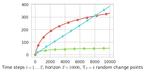
\(\mu = [B(0.1), B(0.2), B(0.3), B(0.4), B(0.5), B(0.6), B(0.7), B(0.8), B(0.9)]\) is an easy problem.
\(\mathrm{UCB}_{\alpha=1/2}\) performs very well here, and EmpiricalMeans is quite inefficient.
[24]:
plotAll(evaluation, 0)
Final ranking for this environment #0 :
- Policy 'UCB($\alpha=0.5$)'    was ranked      1 / 3 for this simulation (last regret = 51.636).
- Policy 'UCB'  was ranked      2 / 3 for this simulation (last regret = 330.67).
- Policy 'EmpiricalMeans'       was ranked      3 / 3 for this simulation (last regret = 384.94).
---------------------------------------------------------------------------
ModuleNotFoundError                       Traceback (most recent call last)
<ipython-input-24-2a63b4dfab0c> in <module>
----> 1 plotAll(evaluation, 0)

<ipython-input-15-8b5020fc41bc> in plotAll(evaluation, envId)
      1 def plotAll(evaluation, envId):
      2     evaluation.printFinalRanking(envId)
----> 3     evaluation.plotRegrets(envId)
      4     evaluation.plotRegrets(envId, semilogx=True)
      5     evaluation.plotRegrets(envId, meanRegret=True)

/tmp/SMPyBandits/notebooks/venv3/lib/python3.6/site-packages/SMPyBandits/Environment/Evaluator.py in plotRegrets(self, envId, savefig, meanReward, plotSTD, plotMaxMin, semilogx, semilogy, loglog, normalizedRegret, drawUpperBound, moreAccurate)
    552         self._xlabel(envId, r"Time steps $t = 1...T$, horizon $T = {}${}".format(self.horizon, self.signature))
    553         lowerbound = self.envs[envId].lowerbound()
--> 554         lowerbound_sparse = self.envs[envId].lowerbound_sparse()
    555         if not (semilogx or semilogy or loglog):
    556             print("\nThis MAB problem has: \n - a [Lai & Robbins] complexity constant C(mu) = {:.3g} for 1-player problem... \n - a Optimal Arm Identification factor H_OI(mu) = {:.2%} ...".format(lowerbound, self.envs[envId].hoifactor()))  # DEBUG

/tmp/SMPyBandits/notebooks/venv3/lib/python3.6/site-packages/SMPyBandits/Environment/MAB.py in lowerbound_sparse(self, sparsity)
    261
    262         try:
--> 263             from Policies.OSSB import solve_optimization_problem__sparse_bandits
    264             ci = solve_optimization_problem__sparse_bandits(self.means, sparsity=sparsity, only_strong_or_weak=False)
    265             # now we use these ci to compute the lower-bound

ModuleNotFoundError: No module named 'Policies'
Second problem
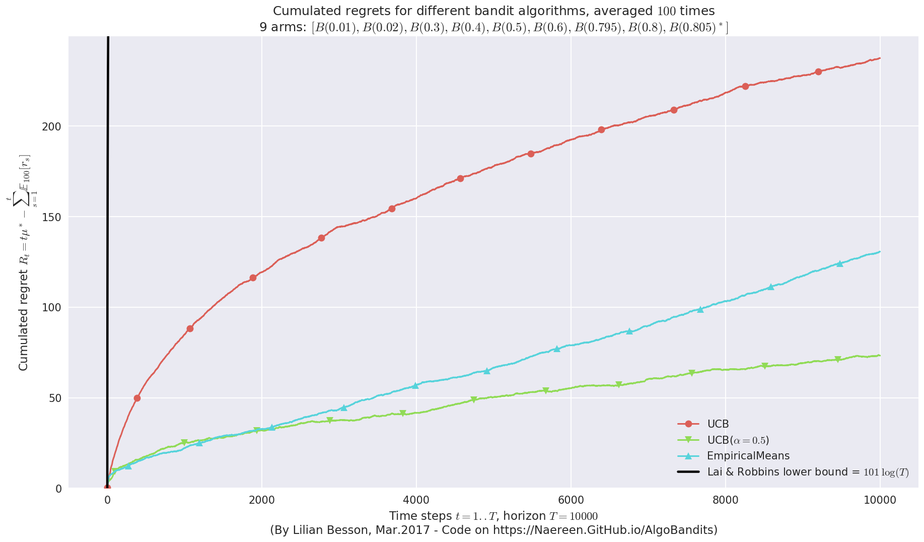
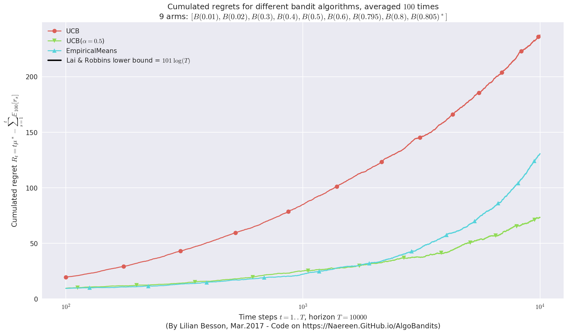
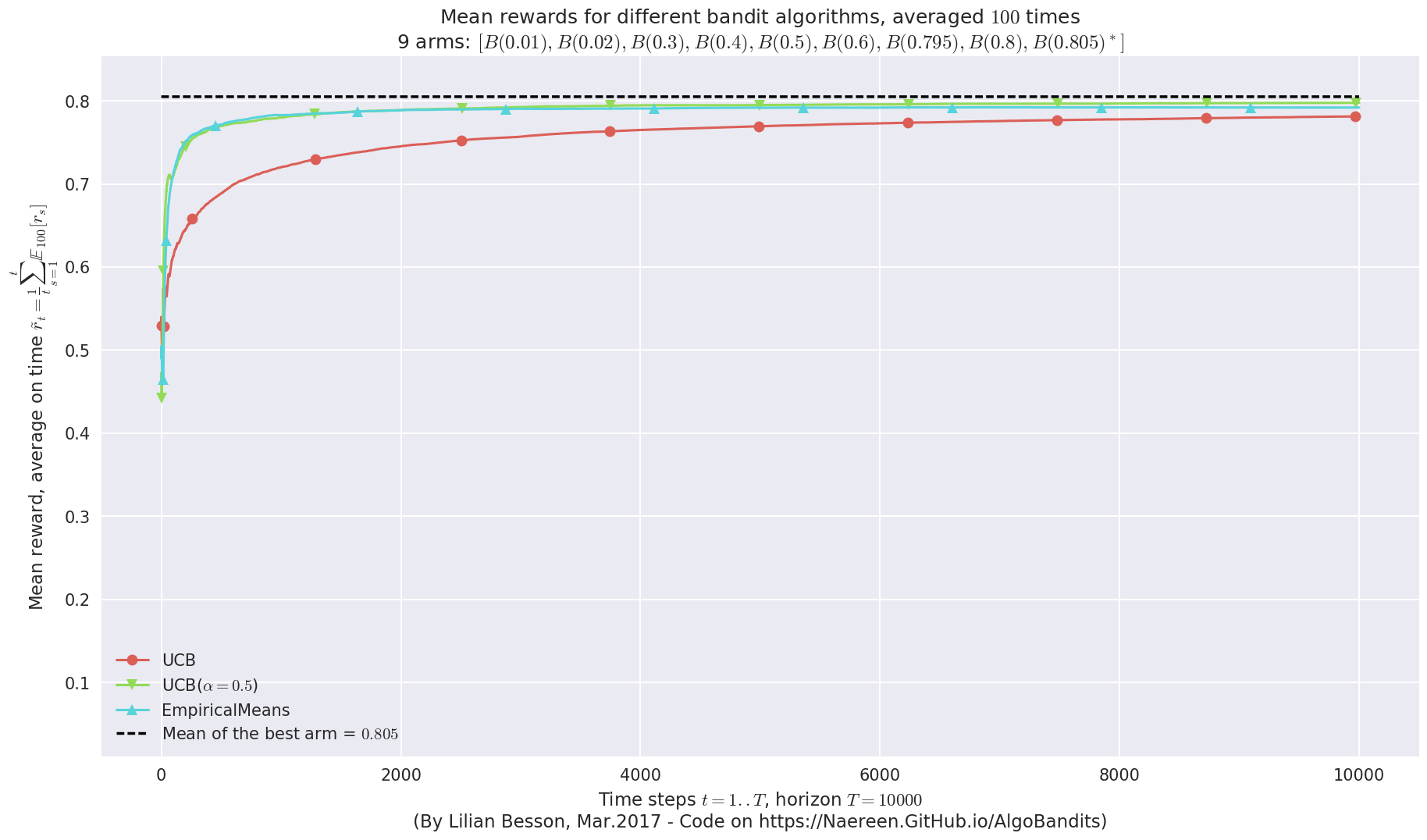
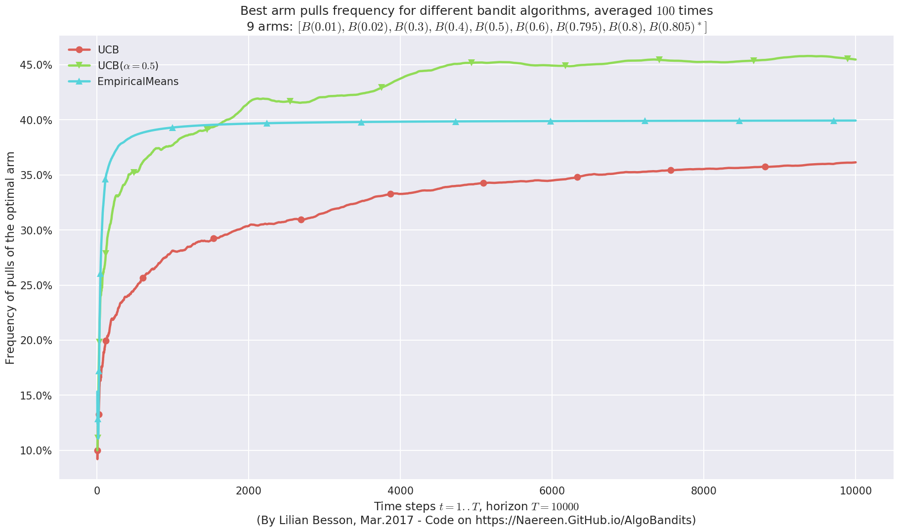
\(\mu = [B(0.01), B(0.02), B(0.3), B(0.4), B(0.5), B(0.6), B(0.795), B(0.8), B(0.805)]\) is harder. There is \(3\) good arms, very close in term of mean rewards.
We could think that EmpiricalMeans will perform even more poorly here, but in fact although \(\mathrm{UCB}_{\alpha=1/2}\) is more efficient in term of best arm identification, EmpiricalMeans is better in term of rewards as it simply focussed on the best arms, without trying to differente between the best \(3\) arms.
[17]:
plotAll(evaluation, 1)
Final ranking for this environment #1 :
- Policy 'UCB($\alpha=0.5$)'    was ranked      1 / 3 for this simulation (last regret = 72.965).
- Policy 'EmpiricalMeans'       was ranked      2 / 3 for this simulation (last regret = 129.855).
- Policy 'UCB'  was ranked      3 / 3 for this simulation (last regret = 236.885).

This MAB problem has:
 - a [Lai & Robbins] complexity constant C(mu) = 101 for 1-player problem...
 - a Optimal Arm Identification factor H_OI(mu) = 55.39% ...
This MAB problem has:
 - a [Lai & Robbins] complexity constant C(mu) = 101 for 1-player problem...
 - a Optimal Arm Identification factor H_OI(mu) = 55.39% ...
This MAB problem has:
 - a [Lai & Robbins] complexity constant C(mu) = 101 for 1-player problem...
 - a Optimal Arm Identification factor H_OI(mu) = 55.39% ...
Third problem
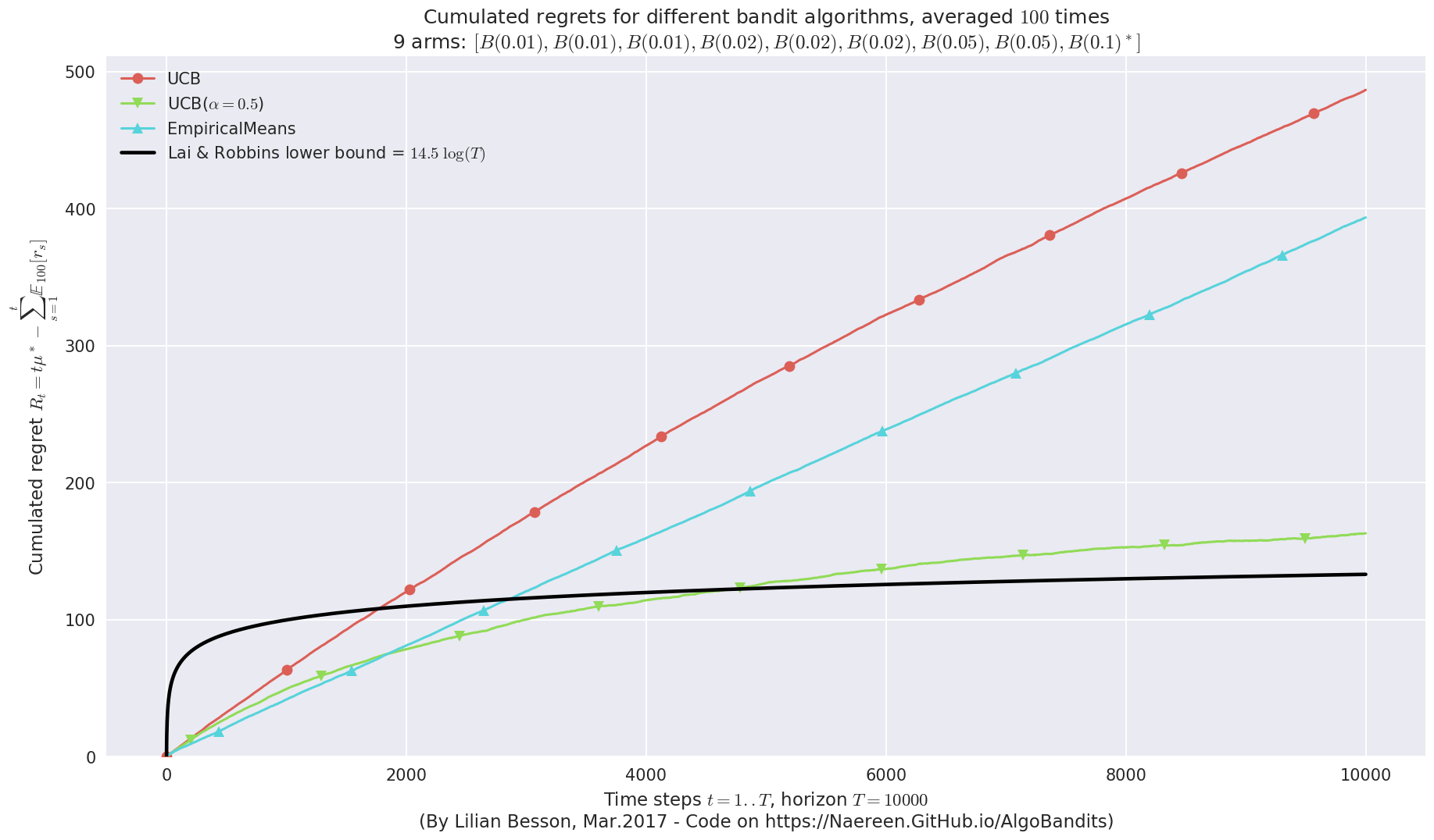
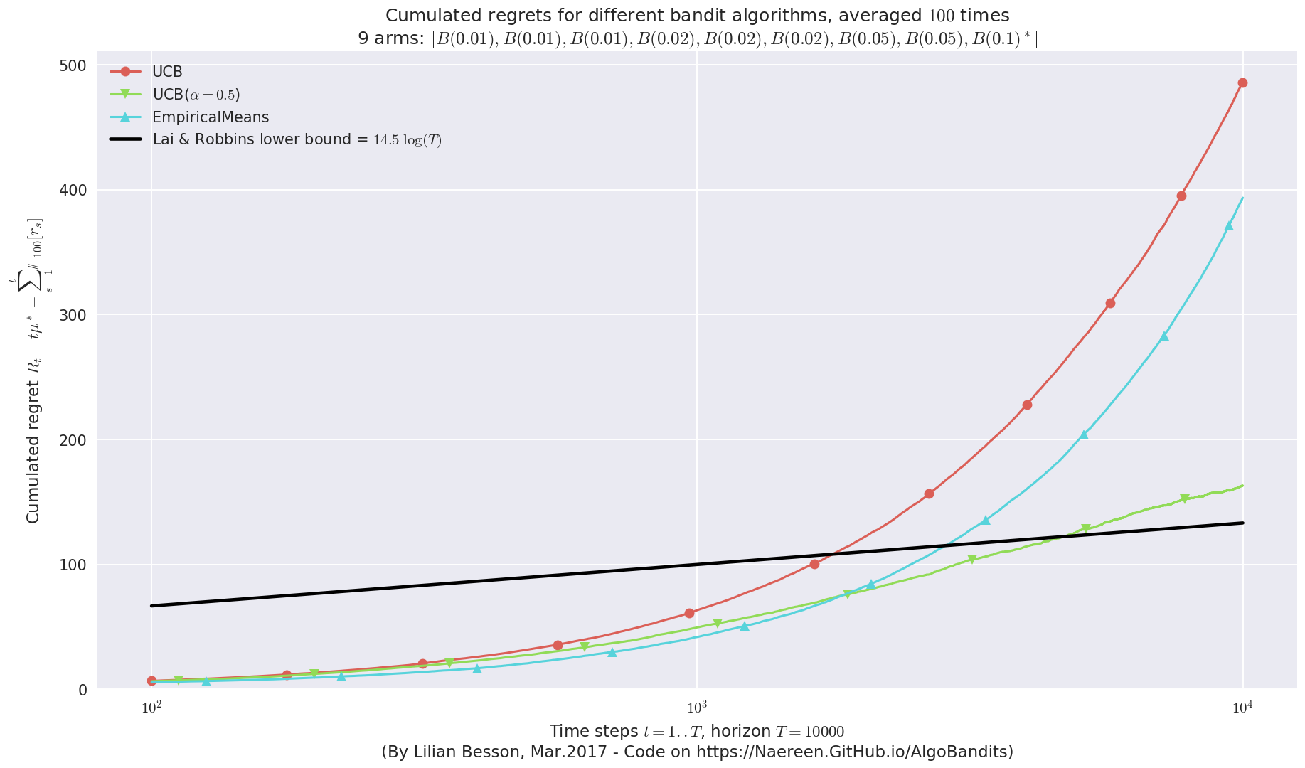
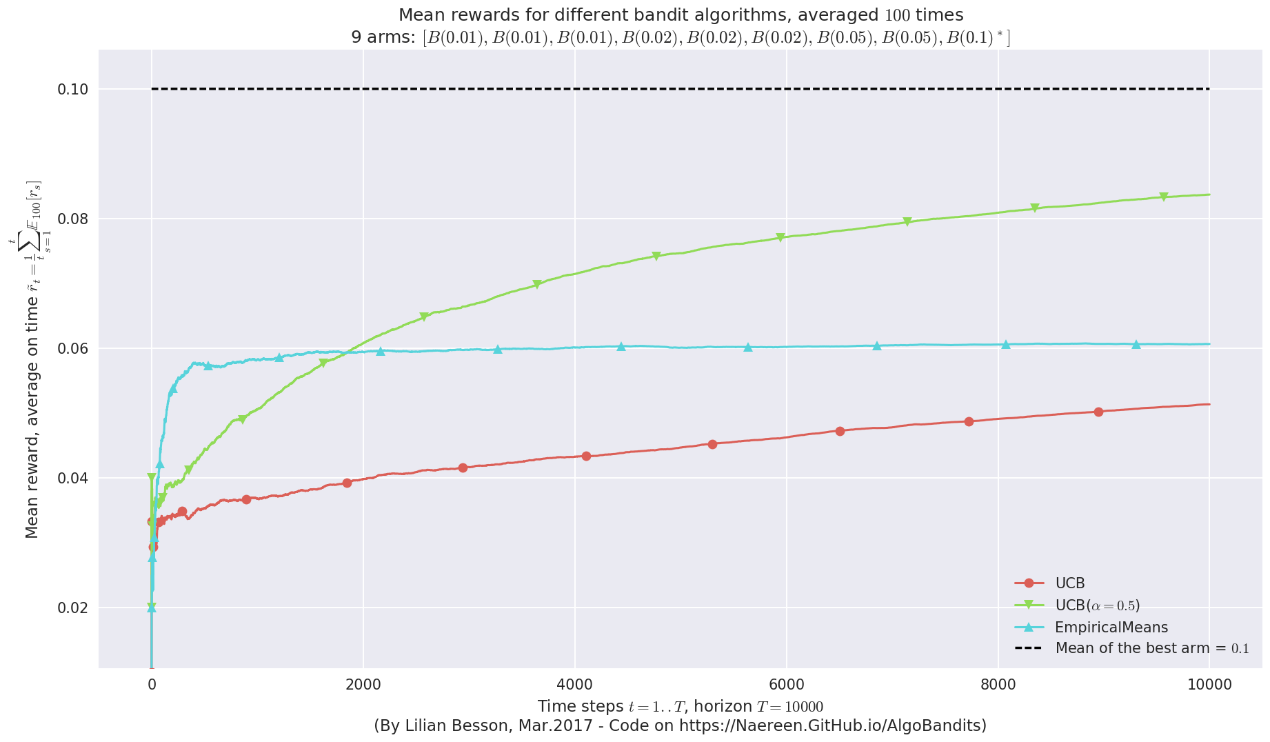
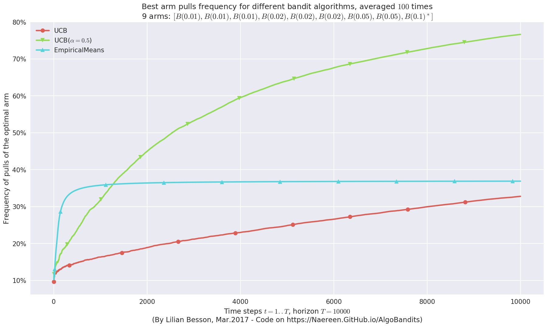
\(\mu = [B(0.01), B(0.01), B(0.01), B(0.02), B(0.02), B(0.02), B(0.05), B(0.05), B(0.1)]\) is another “hard” problem.
This time, EmpiricalMeans is clearly worse than UCBalpha.
[18]:
plotAll(evaluation, 2)
Final ranking for this environment #2 :
- Policy 'UCB($\alpha=0.5$)'    was ranked      1 / 3 for this simulation (last regret = 162.84).
- Policy 'EmpiricalMeans'       was ranked      2 / 3 for this simulation (last regret = 391.55).
- Policy 'UCB'  was ranked      3 / 3 for this simulation (last regret = 484.38).

This MAB problem has:
 - a [Lai & Robbins] complexity constant C(mu) = 14.5 for 1-player problem...
 - a Optimal Arm Identification factor H_OI(mu) = 82.11% ...
This MAB problem has:
 - a [Lai & Robbins] complexity constant C(mu) = 14.5 for 1-player problem...
 - a Optimal Arm Identification factor H_OI(mu) = 82.11% ...
This MAB problem has:
 - a [Lai & Robbins] complexity constant C(mu) = 14.5 for 1-player problem...
 - a Optimal Arm Identification factor H_OI(mu) = 82.11% ...
Conclusion
This small notebook presented the Multi-Armed Bandit problem, as well as the well-known UCB policy, and a simpler policy just based on empirical means.
We illustrated and compared the performance of two UCB algorithms against EmpiricalMeans, on 3 different Bernoulli problems, and it appeared clearly that the confidence bound term in UCB is really useful, even for extremely simple Bernoulli problems.
That’s it for this demo!