Table of Contents
1 An example of a small Multi-Player simulation, with rhoRand and Selfish, for different algorithms
1.1 Creating the problem
1.1.1 Parameters for the simulation
1.1.2 Three MAB problems with Bernoulli arms
1.1.3 Some RL algorithms
1.2 Creating the EvaluatorMultiPlayers objects
1.3 Solving the problem
1.4 Plotting the results
1.4.1 First problem
1.4.2 Second problem
1.4.3 Third problem
1.4.4 Comparing their performances
An example of a small Multi-Player simulation, with rhoRand and Selfish, for different algorithms
First, be sure to be in the main folder, and import
EvaluatorMultiPlayers from Environment package:
In [1]:
from sys import path
path.insert(0, '..')
In [3]:
# Local imports
from Environment import EvaluatorMultiPlayers, tqdm
We also need arms, for instance Bernoulli-distributed arm:
In [6]:
# Import arms
from Arms import Bernoulli
And finally we need some single-player and multi-player Reinforcement Learning algorithms:
In [8]:
# Import algorithms
from Policies import *
from PoliciesMultiPlayers import *
In [9]:
# Just improving the ?? in Jupyter. Thanks to https://nbviewer.jupyter.org/gist/minrk/7715212
from __future__ import print_function
from IPython.core import page
def myprint(s):
    try:
        print(s['text/plain'])
    except (KeyError, TypeError):
        print(s)
page.page = myprint
For instance, this imported the Thompson algorithm:
In [10]:
Thompson?
Init signature: Thompson(nbArms, posterior=<class 'Policies.Beta.Beta'>, lower=0.0, amplitude=1.0)
Docstring:
The Thompson (Bayesian) index policy. By default, it uses a Beta posterior.
Reference: [Thompson - Biometrika, 1933].
Init docstring:
New generic index policy.

- nbArms: the number of arms,
- lower, amplitude: lower value and known amplitude of the rewards.
File:           ~/ownCloud/cloud.openmailbox.org/Thèse_2016-17/src/SMPyBandits.git/Policies/Thompson.py
Type:           type
As well as the rhoRand and Selfish multi-player policy:
In [11]:
rhoRand?
Init signature: rhoRand(nbPlayers, playerAlgo, nbArms, lower=0.0, amplitude=1.0, maxRank=None, *args, **kwargs)
Docstring:
rhoRand: implementation of the multi-player policy from [Distributed Algorithms for Learning..., Anandkumar et al., 2010](http://ieeexplore.ieee.org/document/5462144/).

Init docstring:
- nbPlayers: number of players to create (in self._players).
- playerAlgo: class to use for every players.
- nbArms: number of arms, given as first argument to playerAlgo.
- maxRank: maximum rank allowed by the rhoRand child (default to nbPlayers, but for instance if there is 2 × rhoRand[UCB] + 2 × rhoRand[klUCB], maxRank should be 4 not 2).
- `*args`, `**kwargs`: arguments, named arguments, given to playerAlgo.

Example:

>>> s = rhoRand(nbPlayers, Thompson, nbArms)

- To get a list of usable players, use s.children.
- Warning: s._players is for internal use ONLY!
File:           ~/ownCloud/cloud.openmailbox.org/Thèse_2016-17/src/SMPyBandits.git/PoliciesMultiPlayers/rhoRand.py
Type:           type
In [12]:
Selfish?
Init signature: Selfish(nbPlayers, playerAlgo, nbArms, penalty=None, lower=0.0, amplitude=1.0, *args, **kwargs)
Docstring:
Selfish: a multi-player policy where every player is selfish, playing on their side.

- without nowing how many players there is, and
- not even knowing that they should try to avoid collisions. When a collision happens, the algorithm simply receives a 0 reward for the chosen arm (can be changed with penalty= argument).
Init docstring:
- nbPlayers: number of players to create (in self._players).
- playerAlgo: class to use for every players.
- nbArms: number of arms, given as first argument to playerAlgo.
- `*args`, `**kwargs`: arguments, named arguments, given to playerAlgo.

Examples:

>>> s = Selfish(10, TakeFixedArm, 14)
>>> s = Selfish(NB_PLAYERS, Softmax, nbArms, temperature=TEMPERATURE)

- To get a list of usable players, use s.children.
- Warning: s._players is for internal use ONLY!
File:           ~/ownCloud/cloud.openmailbox.org/Thèse_2016-17/src/SMPyBandits.git/PoliciesMultiPlayers/Selfish.py
Type:           type
We also need a collision model. The usual ones are defined in the
CollisionModels package, and the only one we need is the classical
one, where two or more colliding users don’t receive any rewards.
In [14]:
# Collision Models
from Environment.CollisionModels import onlyUniqUserGetsReward

onlyUniqUserGetsReward?
Signature: onlyUniqUserGetsReward(t, arms, players, choices, rewards, pulls, collisions)
Docstring:
Simple collision model where only the players alone on one arm samples it and receives the reward.

- This is the default collision model, cf. https://arxiv.org/abs/0910.2065v3 collision model 1.
- The numpy array 'choices' is increased according to the number of users who collided (it is NOT binary).
File:      ~/ownCloud/cloud.openmailbox.org/Thèse_2016-17/src/SMPyBandits.git/Environment/CollisionModels.py
Type:      function
Creating the problem
Parameters for the simulation
- \(T = 10000\) is the time horizon,
- \(N = 100\) is the number of repetitions (should be larger to have consistent results),
- \(M = 2\) is the number of players,
N_JOBS = 4is the number of cores used to parallelize the code.
In [17]:
HORIZON = 10000
REPETITIONS = 100
NB_PLAYERS = 2
N_JOBS = 4
collisionModel = onlyUniqUserGetsReward
Three MAB problems with Bernoulli arms
We consider in this example \(3\) problems, with Bernoulli arms,
of different means.
The first problem is very easy, with two good arms and three arms, with a fixed gap \(\Delta = \max_{\mu_i \neq \mu_j}(\mu_{i} - \mu_{j}) = 0.1\).
The second problem is as easier, with a larger gap.
Third problem is harder, with a smaller gap, and a very large difference between the two optimal arms and the suboptimal arms.
Note: right now, the multi-environments evaluator does not work well for MP policies, if there is a number different of arms in the scenarios. So I use the same number of arms in all the problems.
In [18]:
ENVIRONMENTS = [  # 1)  Bernoulli arms
        {   # Scenario 1 from [Komiyama, Honda, Nakagawa, 2016, arXiv 1506.00779]
            "arm_type": Bernoulli,
            "params": [0.3, 0.4, 0.5, 0.6, 0.7]
        },
        {   # Classical scenario
             "arm_type": Bernoulli,
             "params": [0.1, 0.3, 0.5, 0.7, 0.9]
        },
        {   # Harder scenario
             "arm_type": Bernoulli,
             "params": [0.005, 0.01, 0.015, 0.84, 0.85]
        }
    ]
Some RL algorithms
We will use Thompson Sampling, \(\mathrm{UCB}_1\) and \(\mathrm{kl}\)-\(\mathrm{UCB}\), using two different decentralized policy:
rhoRand: each player starts with a rank \(1\), and on collision it selects a new rank \(r \sim U([1,M])\). Instead of aiming at the best arm, each player aims at the \(r\)-th best arm (as given by its UCB index, or posterior sampling if Thompson sampling).Selfish: each player runs a classical RL algorithm, on the joint reward \(\tilde{r}\):\[ \begin{align}\begin{aligned}\tilde{r}_j(t) = r_j(t) \times (1 - \eta_j(t))\\where :math:`r_j(t)` is the reward from the sensing of the\end{aligned}\end{align} \]\(j\)-th arm at time \(t \geq 1\) and \(\eta_j(t)\) is a boolean indicator saying that there were a collision on that arm at time \(t\). In other words, if a player chose arm \(j\) and was alone on it, it receives \(r_j(t)\), and if it was not alone, all players who chose arm \(j\) receive \(0\).
In [19]:
nbArms = len(ENVIRONMENTS[0]['params'])
nbArms

SUCCESSIVE_PLAYERS = [
    # UCB alpha=1
    rhoRand(NB_PLAYERS, UCBalpha, nbArms, alpha=1).children,
    Selfish(NB_PLAYERS, UCBalpha, nbArms, alpha=1).children,
    # Thompson Sampling
    rhoRand(NB_PLAYERS, Thompson, nbArms).children,
    Selfish(NB_PLAYERS, Thompson, nbArms).children,
    # Thompson Sampling
    rhoRand(NB_PLAYERS, klUCB, nbArms).children,
    Selfish(NB_PLAYERS, klUCB, nbArms).children,
]
SUCCESSIVE_PLAYERS
Out[19]:
5
Out[19]:
[[rhoRand(UCB($\alpha=1$)), rhoRand(UCB($\alpha=1$))],
 [Selfish(UCB($\alpha=1$)), Selfish(UCB($\alpha=1$))],
 [rhoRand(Thompson), rhoRand(Thompson)],
 [Selfish(Thompson), Selfish(Thompson)],
 [rhoRand(KL-UCB(Bern)), rhoRand(KL-UCB(Bern))],
 [Selfish(KL-UCB(Bern)), Selfish(KL-UCB(Bern))]]
The mother class in this case does not do any centralized learning, as
Selfish and rhoRand are fully decentralized scenario.
In [20]:
OneMother = SUCCESSIVE_PLAYERS[0][0].mother
OneMother
OneMother.nbArms

OnePlayer = SUCCESSIVE_PLAYERS[0][0]
OnePlayer.nbArms
Out[20]:
<PoliciesMultiPlayers.rhoRand.rhoRand at 0x7f60f06c6470>
Out[20]:
5
Out[20]:
5
Complete configuration for the problem:
In [21]:
configuration = {
    # --- Duration of the experiment
    "horizon": HORIZON,
    # --- Number of repetition of the experiment (to have an average)
    "repetitions": REPETITIONS,
    # --- Parameters for the use of joblib.Parallel
    "n_jobs": N_JOBS,    # = nb of CPU cores
    "verbosity": 6,      # Max joblib verbosity
    # --- Collision model
    "collisionModel": onlyUniqUserGetsReward,
    # --- Arms
    "environment": ENVIRONMENTS,
    # --- Algorithms
    "successive_players": SUCCESSIVE_PLAYERS,
}
Creating the EvaluatorMultiPlayers objects
We will need to create several objects, as the simulation first runs one policy against each environment, and then aggregate them to compare them.
In [22]:
%%time
N_players = len(configuration["successive_players"])

# List to keep all the EvaluatorMultiPlayers objects
evs = [None] * N_players
evaluators = [[None] * N_players] * len(configuration["environment"])

for playersId, players in tqdm(enumerate(configuration["successive_players"]), desc="Creating"):
    print("\n\nConsidering the list of players :\n", players)
    conf = configuration.copy()
    conf['players'] = players
    evs[playersId] = EvaluatorMultiPlayers(conf)
Considering the list of players :
 [rhoRand(UCB($\alpha=1$)), rhoRand(UCB($\alpha=1$))]
Number of players in the multi-players game: 2
Time horizon: 10000
Number of repetitions: 100
Sampling rate for saving, delta_t_save: 1
Sampling rate for plotting, delta_t_plot: 1
Number of jobs for parallelization: 4
Using collision model onlyUniqUserGetsReward (function <function onlyUniqUserGetsReward at 0x7f60f6083510>).
More details:
 Simple collision model where only the players alone on one arm samples it and receives the reward.

    - This is the default collision model, cf. https://arxiv.org/abs/0910.2065v3 collision model 1.
    - The numpy array 'choices' is increased according to the number of users who collided (it is NOT binary).

Creating a new MAB problem ...
  Reading arms of this MAB problem from a dictionnary 'configuration' = {'arm_type': <class 'Arms.Bernoulli.Bernoulli'>, 'params': [0.3, 0.4, 0.5, 0.6, 0.7]} ...
 - with 'arm_type' = <class 'Arms.Bernoulli.Bernoulli'>
 - with 'params' = [0.3, 0.4, 0.5, 0.6, 0.7]
 - with 'arms' = [B(0.3), B(0.4), B(0.5), B(0.6), B(0.7)]
 - with 'means' = [ 0.3  0.4  0.5  0.6  0.7]
 - with 'nbArms' = 5
 - with 'maxArm' = 0.7
 - with 'minArm' = 0.3

This MAB problem has:
 - a [Lai & Robbins] complexity constant C(mu) = 9.46 ...
 - a Optimal Arm Identification factor H_OI(mu) = 60.00% ...
 - with 'arms' represented as: $[B(0.3), B(0.4), B(0.5), B(0.6), B(0.7)^*]$
Creating a new MAB problem ...
  Reading arms of this MAB problem from a dictionnary 'configuration' = {'arm_type': <class 'Arms.Bernoulli.Bernoulli'>, 'params': [0.1, 0.3, 0.5, 0.7, 0.9]} ...
 - with 'arm_type' = <class 'Arms.Bernoulli.Bernoulli'>
 - with 'params' = [0.1, 0.3, 0.5, 0.7, 0.9]
 - with 'arms' = [B(0.1), B(0.3), B(0.5), B(0.7), B(0.9)]
 - with 'means' = [ 0.1  0.3  0.5  0.7  0.9]
 - with 'nbArms' = 5
 - with 'maxArm' = 0.9
 - with 'minArm' = 0.1

This MAB problem has:
 - a [Lai & Robbins] complexity constant C(mu) = 3.12 ...
 - a Optimal Arm Identification factor H_OI(mu) = 40.00% ...
 - with 'arms' represented as: $[B(0.1), B(0.3), B(0.5), B(0.7), B(0.9)^*]$
Creating a new MAB problem ...
  Reading arms of this MAB problem from a dictionnary 'configuration' = {'arm_type': <class 'Arms.Bernoulli.Bernoulli'>, 'params': [0.005, 0.01, 0.015, 0.84, 0.85]} ...
 - with 'arm_type' = <class 'Arms.Bernoulli.Bernoulli'>
 - with 'params' = [0.005, 0.01, 0.015, 0.84, 0.85]
 - with 'arms' = [B(0.005), B(0.01), B(0.015), B(0.84), B(0.85)]
 - with 'means' = [ 0.005  0.01   0.015  0.84   0.85 ]
 - with 'nbArms' = 5
 - with 'maxArm' = 0.85
 - with 'minArm' = 0.005

This MAB problem has:
 - a [Lai & Robbins] complexity constant C(mu) = 27.3 ...
 - a Optimal Arm Identification factor H_OI(mu) = 29.40% ...
 - with 'arms' represented as: $[B(0.005), B(0.01), B(0.015), B(0.84), B(0.85)^*]$
Number of environments to try: 3


Considering the list of players :
 [Selfish(UCB($\alpha=1$)), Selfish(UCB($\alpha=1$))]
Number of players in the multi-players game: 2
Time horizon: 10000
Number of repetitions: 100
Sampling rate for saving, delta_t_save: 1
Sampling rate for plotting, delta_t_plot: 1
Number of jobs for parallelization: 4
Using collision model onlyUniqUserGetsReward (function <function onlyUniqUserGetsReward at 0x7f60f6083510>).
More details:
 Simple collision model where only the players alone on one arm samples it and receives the reward.

    - This is the default collision model, cf. https://arxiv.org/abs/0910.2065v3 collision model 1.
    - The numpy array 'choices' is increased according to the number of users who collided (it is NOT binary).

Creating a new MAB problem ...
  Reading arms of this MAB problem from a dictionnary 'configuration' = {'arm_type': <class 'Arms.Bernoulli.Bernoulli'>, 'params': [0.3, 0.4, 0.5, 0.6, 0.7]} ...
 - with 'arm_type' = <class 'Arms.Bernoulli.Bernoulli'>
 - with 'params' = [0.3, 0.4, 0.5, 0.6, 0.7]
 - with 'arms' = [B(0.3), B(0.4), B(0.5), B(0.6), B(0.7)]
 - with 'means' = [ 0.3  0.4  0.5  0.6  0.7]
 - with 'nbArms' = 5
 - with 'maxArm' = 0.7
 - with 'minArm' = 0.3

This MAB problem has:
 - a [Lai & Robbins] complexity constant C(mu) = 9.46 ...
 - a Optimal Arm Identification factor H_OI(mu) = 60.00% ...
 - with 'arms' represented as: $[B(0.3), B(0.4), B(0.5), B(0.6), B(0.7)^*]$
Creating a new MAB problem ...
  Reading arms of this MAB problem from a dictionnary 'configuration' = {'arm_type': <class 'Arms.Bernoulli.Bernoulli'>, 'params': [0.1, 0.3, 0.5, 0.7, 0.9]} ...
 - with 'arm_type' = <class 'Arms.Bernoulli.Bernoulli'>
 - with 'params' = [0.1, 0.3, 0.5, 0.7, 0.9]
 - with 'arms' = [B(0.1), B(0.3), B(0.5), B(0.7), B(0.9)]
 - with 'means' = [ 0.1  0.3  0.5  0.7  0.9]
 - with 'nbArms' = 5
 - with 'maxArm' = 0.9
 - with 'minArm' = 0.1

This MAB problem has:
 - a [Lai & Robbins] complexity constant C(mu) = 3.12 ...
 - a Optimal Arm Identification factor H_OI(mu) = 40.00% ...
 - with 'arms' represented as: $[B(0.1), B(0.3), B(0.5), B(0.7), B(0.9)^*]$
Creating a new MAB problem ...
  Reading arms of this MAB problem from a dictionnary 'configuration' = {'arm_type': <class 'Arms.Bernoulli.Bernoulli'>, 'params': [0.005, 0.01, 0.015, 0.84, 0.85]} ...
 - with 'arm_type' = <class 'Arms.Bernoulli.Bernoulli'>
 - with 'params' = [0.005, 0.01, 0.015, 0.84, 0.85]
 - with 'arms' = [B(0.005), B(0.01), B(0.015), B(0.84), B(0.85)]
 - with 'means' = [ 0.005  0.01   0.015  0.84   0.85 ]
 - with 'nbArms' = 5
 - with 'maxArm' = 0.85
 - with 'minArm' = 0.005

This MAB problem has:
 - a [Lai & Robbins] complexity constant C(mu) = 27.3 ...
 - a Optimal Arm Identification factor H_OI(mu) = 29.40% ...
 - with 'arms' represented as: $[B(0.005), B(0.01), B(0.015), B(0.84), B(0.85)^*]$
Number of environments to try: 3


Considering the list of players :
 [rhoRand(Thompson), rhoRand(Thompson)]
Number of players in the multi-players game: 2
Time horizon: 10000
Number of repetitions: 100
Sampling rate for saving, delta_t_save: 1
Sampling rate for plotting, delta_t_plot: 1
Number of jobs for parallelization: 4
Using collision model onlyUniqUserGetsReward (function <function onlyUniqUserGetsReward at 0x7f60f6083510>).
More details:
 Simple collision model where only the players alone on one arm samples it and receives the reward.

    - This is the default collision model, cf. https://arxiv.org/abs/0910.2065v3 collision model 1.
    - The numpy array 'choices' is increased according to the number of users who collided (it is NOT binary).

Creating a new MAB problem ...
  Reading arms of this MAB problem from a dictionnary 'configuration' = {'arm_type': <class 'Arms.Bernoulli.Bernoulli'>, 'params': [0.3, 0.4, 0.5, 0.6, 0.7]} ...
 - with 'arm_type' = <class 'Arms.Bernoulli.Bernoulli'>
 - with 'params' = [0.3, 0.4, 0.5, 0.6, 0.7]
 - with 'arms' = [B(0.3), B(0.4), B(0.5), B(0.6), B(0.7)]
 - with 'means' = [ 0.3  0.4  0.5  0.6  0.7]
 - with 'nbArms' = 5
 - with 'maxArm' = 0.7
 - with 'minArm' = 0.3

This MAB problem has:
 - a [Lai & Robbins] complexity constant C(mu) = 9.46 ...
 - a Optimal Arm Identification factor H_OI(mu) = 60.00% ...
 - with 'arms' represented as: $[B(0.3), B(0.4), B(0.5), B(0.6), B(0.7)^*]$
Creating a new MAB problem ...
  Reading arms of this MAB problem from a dictionnary 'configuration' = {'arm_type': <class 'Arms.Bernoulli.Bernoulli'>, 'params': [0.1, 0.3, 0.5, 0.7, 0.9]} ...
 - with 'arm_type' = <class 'Arms.Bernoulli.Bernoulli'>
 - with 'params' = [0.1, 0.3, 0.5, 0.7, 0.9]
 - with 'arms' = [B(0.1), B(0.3), B(0.5), B(0.7), B(0.9)]
 - with 'means' = [ 0.1  0.3  0.5  0.7  0.9]
 - with 'nbArms' = 5
 - with 'maxArm' = 0.9
 - with 'minArm' = 0.1

This MAB problem has:
 - a [Lai & Robbins] complexity constant C(mu) = 3.12 ...
 - a Optimal Arm Identification factor H_OI(mu) = 40.00% ...
 - with 'arms' represented as: $[B(0.1), B(0.3), B(0.5), B(0.7), B(0.9)^*]$
Creating a new MAB problem ...
  Reading arms of this MAB problem from a dictionnary 'configuration' = {'arm_type': <class 'Arms.Bernoulli.Bernoulli'>, 'params': [0.005, 0.01, 0.015, 0.84, 0.85]} ...
 - with 'arm_type' = <class 'Arms.Bernoulli.Bernoulli'>
 - with 'params' = [0.005, 0.01, 0.015, 0.84, 0.85]
 - with 'arms' = [B(0.005), B(0.01), B(0.015), B(0.84), B(0.85)]
 - with 'means' = [ 0.005  0.01   0.015  0.84   0.85 ]
 - with 'nbArms' = 5
 - with 'maxArm' = 0.85
 - with 'minArm' = 0.005

This MAB problem has:
 - a [Lai & Robbins] complexity constant C(mu) = 27.3 ...
 - a Optimal Arm Identification factor H_OI(mu) = 29.40% ...
 - with 'arms' represented as: $[B(0.005), B(0.01), B(0.015), B(0.84), B(0.85)^*]$
Number of environments to try: 3


Considering the list of players :
 [Selfish(Thompson), Selfish(Thompson)]
Number of players in the multi-players game: 2
Time horizon: 10000
Number of repetitions: 100
Sampling rate for saving, delta_t_save: 1
Sampling rate for plotting, delta_t_plot: 1
Number of jobs for parallelization: 4
Using collision model onlyUniqUserGetsReward (function <function onlyUniqUserGetsReward at 0x7f60f6083510>).
More details:
 Simple collision model where only the players alone on one arm samples it and receives the reward.

    - This is the default collision model, cf. https://arxiv.org/abs/0910.2065v3 collision model 1.
    - The numpy array 'choices' is increased according to the number of users who collided (it is NOT binary).

Creating a new MAB problem ...
  Reading arms of this MAB problem from a dictionnary 'configuration' = {'arm_type': <class 'Arms.Bernoulli.Bernoulli'>, 'params': [0.3, 0.4, 0.5, 0.6, 0.7]} ...
 - with 'arm_type' = <class 'Arms.Bernoulli.Bernoulli'>
 - with 'params' = [0.3, 0.4, 0.5, 0.6, 0.7]
 - with 'arms' = [B(0.3), B(0.4), B(0.5), B(0.6), B(0.7)]
 - with 'means' = [ 0.3  0.4  0.5  0.6  0.7]
 - with 'nbArms' = 5
 - with 'maxArm' = 0.7
 - with 'minArm' = 0.3

This MAB problem has:
 - a [Lai & Robbins] complexity constant C(mu) = 9.46 ...
 - a Optimal Arm Identification factor H_OI(mu) = 60.00% ...
 - with 'arms' represented as: $[B(0.3), B(0.4), B(0.5), B(0.6), B(0.7)^*]$
Creating a new MAB problem ...
  Reading arms of this MAB problem from a dictionnary 'configuration' = {'arm_type': <class 'Arms.Bernoulli.Bernoulli'>, 'params': [0.1, 0.3, 0.5, 0.7, 0.9]} ...
 - with 'arm_type' = <class 'Arms.Bernoulli.Bernoulli'>
 - with 'params' = [0.1, 0.3, 0.5, 0.7, 0.9]
 - with 'arms' = [B(0.1), B(0.3), B(0.5), B(0.7), B(0.9)]
 - with 'means' = [ 0.1  0.3  0.5  0.7  0.9]
 - with 'nbArms' = 5
 - with 'maxArm' = 0.9
 - with 'minArm' = 0.1

This MAB problem has:
 - a [Lai & Robbins] complexity constant C(mu) = 3.12 ...
 - a Optimal Arm Identification factor H_OI(mu) = 40.00% ...
 - with 'arms' represented as: $[B(0.1), B(0.3), B(0.5), B(0.7), B(0.9)^*]$
Creating a new MAB problem ...
  Reading arms of this MAB problem from a dictionnary 'configuration' = {'arm_type': <class 'Arms.Bernoulli.Bernoulli'>, 'params': [0.005, 0.01, 0.015, 0.84, 0.85]} ...
 - with 'arm_type' = <class 'Arms.Bernoulli.Bernoulli'>
 - with 'params' = [0.005, 0.01, 0.015, 0.84, 0.85]
 - with 'arms' = [B(0.005), B(0.01), B(0.015), B(0.84), B(0.85)]
 - with 'means' = [ 0.005  0.01   0.015  0.84   0.85 ]
 - with 'nbArms' = 5
 - with 'maxArm' = 0.85
 - with 'minArm' = 0.005

This MAB problem has:
 - a [Lai & Robbins] complexity constant C(mu) = 27.3 ...
 - a Optimal Arm Identification factor H_OI(mu) = 29.40% ...
 - with 'arms' represented as: $[B(0.005), B(0.01), B(0.015), B(0.84), B(0.85)^*]$
Number of environments to try: 3


Considering the list of players :
 [rhoRand(KL-UCB(Bern)), rhoRand(KL-UCB(Bern))]
Number of players in the multi-players game: 2
Time horizon: 10000
Number of repetitions: 100
Sampling rate for saving, delta_t_save: 1
Sampling rate for plotting, delta_t_plot: 1
Number of jobs for parallelization: 4
Using collision model onlyUniqUserGetsReward (function <function onlyUniqUserGetsReward at 0x7f60f6083510>).
More details:
 Simple collision model where only the players alone on one arm samples it and receives the reward.

    - This is the default collision model, cf. https://arxiv.org/abs/0910.2065v3 collision model 1.
    - The numpy array 'choices' is increased according to the number of users who collided (it is NOT binary).

Creating a new MAB problem ...
  Reading arms of this MAB problem from a dictionnary 'configuration' = {'arm_type': <class 'Arms.Bernoulli.Bernoulli'>, 'params': [0.3, 0.4, 0.5, 0.6, 0.7]} ...
 - with 'arm_type' = <class 'Arms.Bernoulli.Bernoulli'>
 - with 'params' = [0.3, 0.4, 0.5, 0.6, 0.7]
 - with 'arms' = [B(0.3), B(0.4), B(0.5), B(0.6), B(0.7)]
 - with 'means' = [ 0.3  0.4  0.5  0.6  0.7]
 - with 'nbArms' = 5
 - with 'maxArm' = 0.7
 - with 'minArm' = 0.3

This MAB problem has:
 - a [Lai & Robbins] complexity constant C(mu) = 9.46 ...
 - a Optimal Arm Identification factor H_OI(mu) = 60.00% ...
 - with 'arms' represented as: $[B(0.3), B(0.4), B(0.5), B(0.6), B(0.7)^*]$
Creating a new MAB problem ...
  Reading arms of this MAB problem from a dictionnary 'configuration' = {'arm_type': <class 'Arms.Bernoulli.Bernoulli'>, 'params': [0.1, 0.3, 0.5, 0.7, 0.9]} ...
 - with 'arm_type' = <class 'Arms.Bernoulli.Bernoulli'>
 - with 'params' = [0.1, 0.3, 0.5, 0.7, 0.9]
 - with 'arms' = [B(0.1), B(0.3), B(0.5), B(0.7), B(0.9)]
 - with 'means' = [ 0.1  0.3  0.5  0.7  0.9]
 - with 'nbArms' = 5
 - with 'maxArm' = 0.9
 - with 'minArm' = 0.1

This MAB problem has:
 - a [Lai & Robbins] complexity constant C(mu) = 3.12 ...
 - a Optimal Arm Identification factor H_OI(mu) = 40.00% ...
 - with 'arms' represented as: $[B(0.1), B(0.3), B(0.5), B(0.7), B(0.9)^*]$
Creating a new MAB problem ...
  Reading arms of this MAB problem from a dictionnary 'configuration' = {'arm_type': <class 'Arms.Bernoulli.Bernoulli'>, 'params': [0.005, 0.01, 0.015, 0.84, 0.85]} ...
 - with 'arm_type' = <class 'Arms.Bernoulli.Bernoulli'>
 - with 'params' = [0.005, 0.01, 0.015, 0.84, 0.85]
 - with 'arms' = [B(0.005), B(0.01), B(0.015), B(0.84), B(0.85)]
 - with 'means' = [ 0.005  0.01   0.015  0.84   0.85 ]
 - with 'nbArms' = 5
 - with 'maxArm' = 0.85
 - with 'minArm' = 0.005

This MAB problem has:
 - a [Lai & Robbins] complexity constant C(mu) = 27.3 ...
 - a Optimal Arm Identification factor H_OI(mu) = 29.40% ...
 - with 'arms' represented as: $[B(0.005), B(0.01), B(0.015), B(0.84), B(0.85)^*]$
Number of environments to try: 3


Considering the list of players :
 [Selfish(KL-UCB(Bern)), Selfish(KL-UCB(Bern))]
Number of players in the multi-players game: 2
Time horizon: 10000
Number of repetitions: 100
Sampling rate for saving, delta_t_save: 1
Sampling rate for plotting, delta_t_plot: 1
Number of jobs for parallelization: 4
Using collision model onlyUniqUserGetsReward (function <function onlyUniqUserGetsReward at 0x7f60f6083510>).
More details:
 Simple collision model where only the players alone on one arm samples it and receives the reward.

    - This is the default collision model, cf. https://arxiv.org/abs/0910.2065v3 collision model 1.
    - The numpy array 'choices' is increased according to the number of users who collided (it is NOT binary).

Creating a new MAB problem ...
  Reading arms of this MAB problem from a dictionnary 'configuration' = {'arm_type': <class 'Arms.Bernoulli.Bernoulli'>, 'params': [0.3, 0.4, 0.5, 0.6, 0.7]} ...
 - with 'arm_type' = <class 'Arms.Bernoulli.Bernoulli'>
 - with 'params' = [0.3, 0.4, 0.5, 0.6, 0.7]
 - with 'arms' = [B(0.3), B(0.4), B(0.5), B(0.6), B(0.7)]
 - with 'means' = [ 0.3  0.4  0.5  0.6  0.7]
 - with 'nbArms' = 5
 - with 'maxArm' = 0.7
 - with 'minArm' = 0.3

This MAB problem has:
 - a [Lai & Robbins] complexity constant C(mu) = 9.46 ...
 - a Optimal Arm Identification factor H_OI(mu) = 60.00% ...
 - with 'arms' represented as: $[B(0.3), B(0.4), B(0.5), B(0.6), B(0.7)^*]$
Creating a new MAB problem ...
  Reading arms of this MAB problem from a dictionnary 'configuration' = {'arm_type': <class 'Arms.Bernoulli.Bernoulli'>, 'params': [0.1, 0.3, 0.5, 0.7, 0.9]} ...
 - with 'arm_type' = <class 'Arms.Bernoulli.Bernoulli'>
 - with 'params' = [0.1, 0.3, 0.5, 0.7, 0.9]
 - with 'arms' = [B(0.1), B(0.3), B(0.5), B(0.7), B(0.9)]
 - with 'means' = [ 0.1  0.3  0.5  0.7  0.9]
 - with 'nbArms' = 5
 - with 'maxArm' = 0.9
 - with 'minArm' = 0.1

This MAB problem has:
 - a [Lai & Robbins] complexity constant C(mu) = 3.12 ...
 - a Optimal Arm Identification factor H_OI(mu) = 40.00% ...
 - with 'arms' represented as: $[B(0.1), B(0.3), B(0.5), B(0.7), B(0.9)^*]$
Creating a new MAB problem ...
  Reading arms of this MAB problem from a dictionnary 'configuration' = {'arm_type': <class 'Arms.Bernoulli.Bernoulli'>, 'params': [0.005, 0.01, 0.015, 0.84, 0.85]} ...
 - with 'arm_type' = <class 'Arms.Bernoulli.Bernoulli'>
 - with 'params' = [0.005, 0.01, 0.015, 0.84, 0.85]
 - with 'arms' = [B(0.005), B(0.01), B(0.015), B(0.84), B(0.85)]
 - with 'means' = [ 0.005  0.01   0.015  0.84   0.85 ]
 - with 'nbArms' = 5
 - with 'maxArm' = 0.85
 - with 'minArm' = 0.005

This MAB problem has:
 - a [Lai & Robbins] complexity constant C(mu) = 27.3 ...
 - a Optimal Arm Identification factor H_OI(mu) = 29.40% ...
 - with 'arms' represented as: $[B(0.005), B(0.01), B(0.015), B(0.84), B(0.85)^*]$
Number of environments to try: 3

CPU times: user 240 ms, sys: 16 ms, total: 256 ms
Wall time: 333 ms
Solving the problem
Now we can simulate the \(2\) environments, for the successive policies. That part can take some time.
In [23]:
%%time
for playersId, evaluation in tqdm(enumerate(evs), desc="Policies"):
    for envId, env in tqdm(enumerate(evaluation.envs), desc="Problems"):
        # Evaluate just that env
        evaluation.startOneEnv(envId, env)
        # Storing it after simulation is done
        evaluators[envId][playersId] = evaluation
Evaluating environment: MAB(nbArms: 5, arms: [B(0.3), B(0.4), B(0.5), B(0.6), B(0.7)], minArm: 0.3, maxArm: 0.7)
- Adding player #1 = #1<$\rho^{\mathrm{Rand}}$[UCB($\alpha=1$)]> ...
  Using this already created player 'player' = #1<$\rho^{\mathrm{Rand}}$[UCB($\alpha=1$)]> ...
- Adding player #2 = #2<$\rho^{\mathrm{Rand}}$[UCB($\alpha=1$)]> ...
  Using this already created player 'player' = #2<$\rho^{\mathrm{Rand}}$[UCB($\alpha=1$)]> ...
Estimated order by the policy #1<$\rho^{\mathrm{Rand}}$[UCB($\alpha=1$), rank:2]> after 10000 steps: [0 2 1 3 4] ...
  ==> Optimal arm identification: 100.00% (relative success)...
  ==> Manhattan   distance from optimal ordering: 84.00% (relative success)...
  ==> Kendell Tau distance from optimal ordering: 95.00% (relative success)...
  ==> Spearman    distance from optimal ordering: 96.26% (relative success)...
  ==> Gestalt     distance from optimal ordering: 80.00% (relative success)...
  ==> Mean distance from optimal ordering: 88.81% (relative success)...

Estimated order by the policy #2<$\rho^{\mathrm{Rand}}$[UCB($\alpha=1$), rank:2]> after 10000 steps: [0 2 1 4 3] ...
  ==> Optimal arm identification: 100.00% (relative success)...
  ==> Manhattan   distance from optimal ordering: 68.00% (relative success)...
  ==> Kendell Tau distance from optimal ordering: 85.84% (relative success)...
  ==> Spearman    distance from optimal ordering: 89.59% (relative success)...
  ==> Gestalt     distance from optimal ordering: 60.00% (relative success)...
  ==> Mean distance from optimal ordering: 75.86% (relative success)...
[Parallel(n_jobs=4)]: Done   5 tasks      | elapsed:    3.3s
[Parallel(n_jobs=4)]: Done  42 tasks      | elapsed:   16.8s
[Parallel(n_jobs=4)]: Done 100 out of 100 | elapsed:   37.7s finished
Evaluating environment: MAB(nbArms: 5, arms: [B(0.1), B(0.3), B(0.5), B(0.7), B(0.9)], minArm: 0.1, maxArm: 0.9)
- Adding player #1 = #1<$\rho^{\mathrm{Rand}}$[UCB($\alpha=1$)]> ...
  Using this already created player 'player' = #1<$\rho^{\mathrm{Rand}}$[UCB($\alpha=1$)]> ...
- Adding player #2 = #2<$\rho^{\mathrm{Rand}}$[UCB($\alpha=1$)]> ...
  Using this already created player 'player' = #2<$\rho^{\mathrm{Rand}}$[UCB($\alpha=1$)]> ...
Estimated order by the policy #1<$\rho^{\mathrm{Rand}}$[UCB($\alpha=1$), rank:2]> after 10000 steps: [1 2 0 3 4] ...
  ==> Optimal arm identification: 100.00% (relative success)...
  ==> Manhattan   distance from optimal ordering: 68.00% (relative success)...
  ==> Kendell Tau distance from optimal ordering: 85.84% (relative success)...
  ==> Spearman    distance from optimal ordering: 81.19% (relative success)...
  ==> Gestalt     distance from optimal ordering: 80.00% (relative success)...
  ==> Mean distance from optimal ordering: 78.76% (relative success)...

Estimated order by the policy #2<$\rho^{\mathrm{Rand}}$[UCB($\alpha=1$), rank:2]> after 10000 steps: [1 0 3 4 2] ...
  ==> Optimal arm identification: 87.50% (relative success)...
  ==> Manhattan   distance from optimal ordering: 52.00% (relative success)...
  ==> Kendell Tau distance from optimal ordering: 67.28% (relative success)...
  ==> Spearman    distance from optimal ordering: 71.52% (relative success)...
  ==> Gestalt     distance from optimal ordering: 60.00% (relative success)...
  ==> Mean distance from optimal ordering: 62.70% (relative success)...
[Parallel(n_jobs=4)]: Done   5 tasks      | elapsed:    2.9s
[Parallel(n_jobs=4)]: Done  42 tasks      | elapsed:   16.6s
[Parallel(n_jobs=4)]: Done 100 out of 100 | elapsed:   39.2s finished
Evaluating environment: MAB(nbArms: 5, arms: [B(0.005), B(0.01), B(0.015), B(0.84), B(0.85)], minArm: 0.005, maxArm: 0.85)
- Adding player #1 = #1<$\rho^{\mathrm{Rand}}$[UCB($\alpha=1$)]> ...
  Using this already created player 'player' = #1<$\rho^{\mathrm{Rand}}$[UCB($\alpha=1$)]> ...
- Adding player #2 = #2<$\rho^{\mathrm{Rand}}$[UCB($\alpha=1$)]> ...
  Using this already created player 'player' = #2<$\rho^{\mathrm{Rand}}$[UCB($\alpha=1$)]> ...
Estimated order by the policy #1<$\rho^{\mathrm{Rand}}$[UCB($\alpha=1$), rank:2]> after 10000 steps: [0 1 2 3 4] ...
  ==> Optimal arm identification: 100.00% (relative success)...
  ==> Manhattan   distance from optimal ordering: 100.00% (relative success)...
  ==> Kendell Tau distance from optimal ordering: 98.57% (relative success)...
  ==> Spearman    distance from optimal ordering: 100.00% (relative success)...
  ==> Gestalt     distance from optimal ordering: 100.00% (relative success)...
  ==> Mean distance from optimal ordering: 99.64% (relative success)...

Estimated order by the policy #2<$\rho^{\mathrm{Rand}}$[UCB($\alpha=1$), rank:2]> after 10000 steps: [0 1 2 4 3] ...
  ==> Optimal arm identification: 100.00% (relative success)...
  ==> Manhattan   distance from optimal ordering: 84.00% (relative success)...
  ==> Kendell Tau distance from optimal ordering: 95.00% (relative success)...
  ==> Spearman    distance from optimal ordering: 96.26% (relative success)...
  ==> Gestalt     distance from optimal ordering: 80.00% (relative success)...
  ==> Mean distance from optimal ordering: 88.81% (relative success)...
[Parallel(n_jobs=4)]: Done   5 tasks      | elapsed:    3.3s
[Parallel(n_jobs=4)]: Done  42 tasks      | elapsed:   17.7s
[Parallel(n_jobs=4)]: Done 100 out of 100 | elapsed:   36.0s finished
Evaluating environment: MAB(nbArms: 5, arms: [B(0.3), B(0.4), B(0.5), B(0.6), B(0.7)], minArm: 0.3, maxArm: 0.7)
- Adding player #1 = #1<Selfish[UCB($\alpha=1$)]> ...
  Using this already created player 'player' = #1<Selfish[UCB($\alpha=1$)]> ...
- Adding player #2 = #2<Selfish[UCB($\alpha=1$)]> ...
  Using this already created player 'player' = #2<Selfish[UCB($\alpha=1$)]> ...
Estimated order by the policy #1<Selfish[UCB($\alpha=1$)]> after 10000 steps: [1 2 4 0 3] ...
  ==> Optimal arm identification: 69.23% (relative success)...
  ==> Manhattan   distance from optimal ordering: 36.00% (relative success)...
  ==> Kendell Tau distance from optimal ordering: 37.58% (relative success)...
  ==> Spearman    distance from optimal ordering: 25.29% (relative success)...
  ==> Gestalt     distance from optimal ordering: 60.00% (relative success)...
  ==> Mean distance from optimal ordering: 39.72% (relative success)...

Estimated order by the policy #2<Selfish[UCB($\alpha=1$)]> after 10000 steps: [1 0 3 2 4] ...
  ==> Optimal arm identification: 92.31% (relative success)...
  ==> Manhattan   distance from optimal ordering: 68.00% (relative success)...
  ==> Kendell Tau distance from optimal ordering: 85.84% (relative success)...
  ==> Spearman    distance from optimal ordering: 89.59% (relative success)...
  ==> Gestalt     distance from optimal ordering: 60.00% (relative success)...
  ==> Mean distance from optimal ordering: 75.86% (relative success)...
[Parallel(n_jobs=4)]: Done   5 tasks      | elapsed:    2.4s
[Parallel(n_jobs=4)]: Done  42 tasks      | elapsed:   17.9s
[Parallel(n_jobs=4)]: Done 100 out of 100 | elapsed:   36.0s finished
Evaluating environment: MAB(nbArms: 5, arms: [B(0.1), B(0.3), B(0.5), B(0.7), B(0.9)], minArm: 0.1, maxArm: 0.9)
- Adding player #1 = #1<Selfish[UCB($\alpha=1$)]> ...
  Using this already created player 'player' = #1<Selfish[UCB($\alpha=1$)]> ...
- Adding player #2 = #2<Selfish[UCB($\alpha=1$)]> ...
  Using this already created player 'player' = #2<Selfish[UCB($\alpha=1$)]> ...
Estimated order by the policy #1<Selfish[UCB($\alpha=1$)]> after 10000 steps: [4 0 2 1 3] ...
  ==> Optimal arm identification: 62.50% (relative success)...
  ==> Manhattan   distance from optimal ordering: 36.00% (relative success)...
  ==> Kendell Tau distance from optimal ordering: 0.00% (relative success)...
  ==> Spearman    distance from optimal ordering: 12.71% (relative success)...
  ==> Gestalt     distance from optimal ordering: 20.00% (relative success)...
  ==> Mean distance from optimal ordering: 17.18% (relative success)...

Estimated order by the policy #2<Selfish[UCB($\alpha=1$)]> after 10000 steps: [1 3 0 2 4] ...
  ==> Optimal arm identification: 87.50% (relative success)...
  ==> Manhattan   distance from optimal ordering: 52.00% (relative success)...
  ==> Kendell Tau distance from optimal ordering: 67.28% (relative success)...
  ==> Spearman    distance from optimal ordering: 60.90% (relative success)...
  ==> Gestalt     distance from optimal ordering: 60.00% (relative success)...
  ==> Mean distance from optimal ordering: 60.05% (relative success)...
[Parallel(n_jobs=4)]: Done   5 tasks      | elapsed:    2.4s
[Parallel(n_jobs=4)]: Done  42 tasks      | elapsed:   13.7s
[Parallel(n_jobs=4)]: Done 100 out of 100 | elapsed:   33.6s finished
Evaluating environment: MAB(nbArms: 5, arms: [B(0.005), B(0.01), B(0.015), B(0.84), B(0.85)], minArm: 0.005, maxArm: 0.85)
- Adding player #1 = #1<Selfish[UCB($\alpha=1$)]> ...
  Using this already created player 'player' = #1<Selfish[UCB($\alpha=1$)]> ...
- Adding player #2 = #2<Selfish[UCB($\alpha=1$)]> ...
  Using this already created player 'player' = #2<Selfish[UCB($\alpha=1$)]> ...
Estimated order by the policy #1<Selfish[UCB($\alpha=1$)]> after 10000 steps: [0 1 2 4 3] ...
  ==> Optimal arm identification: 100.00% (relative success)...
  ==> Manhattan   distance from optimal ordering: 84.00% (relative success)...
  ==> Kendell Tau distance from optimal ordering: 95.00% (relative success)...
  ==> Spearman    distance from optimal ordering: 96.26% (relative success)...
  ==> Gestalt     distance from optimal ordering: 80.00% (relative success)...
  ==> Mean distance from optimal ordering: 88.81% (relative success)...

Estimated order by the policy #2<Selfish[UCB($\alpha=1$)]> after 10000 steps: [0 1 2 3 4] ...
  ==> Optimal arm identification: 100.00% (relative success)...
  ==> Manhattan   distance from optimal ordering: 100.00% (relative success)...
  ==> Kendell Tau distance from optimal ordering: 98.57% (relative success)...
  ==> Spearman    distance from optimal ordering: 100.00% (relative success)...
  ==> Gestalt     distance from optimal ordering: 100.00% (relative success)...
  ==> Mean distance from optimal ordering: 99.64% (relative success)...
[Parallel(n_jobs=4)]: Done   5 tasks      | elapsed:    2.9s
[Parallel(n_jobs=4)]: Done  42 tasks      | elapsed:   14.8s
[Parallel(n_jobs=4)]: Done 100 out of 100 | elapsed:   32.0s finished
Evaluating environment: MAB(nbArms: 5, arms: [B(0.3), B(0.4), B(0.5), B(0.6), B(0.7)], minArm: 0.3, maxArm: 0.7)
- Adding player #1 = #1<$\rho^{\mathrm{Rand}}$[Thompson]> ...
  Using this already created player 'player' = #1<$\rho^{\mathrm{Rand}}$[Thompson]> ...
- Adding player #2 = #2<$\rho^{\mathrm{Rand}}$[Thompson]> ...
  Using this already created player 'player' = #2<$\rho^{\mathrm{Rand}}$[Thompson]> ...
Estimated order by the policy #1<$\rho^{\mathrm{Rand}}$[Thompson, rank:2]> after 10000 steps: [0 1 2 3 4] ...
  ==> Optimal arm identification: 100.00% (relative success)...
  ==> Manhattan   distance from optimal ordering: 100.00% (relative success)...
  ==> Kendell Tau distance from optimal ordering: 98.57% (relative success)...
  ==> Spearman    distance from optimal ordering: 100.00% (relative success)...
  ==> Gestalt     distance from optimal ordering: 100.00% (relative success)...
  ==> Mean distance from optimal ordering: 99.64% (relative success)...

Estimated order by the policy #2<$\rho^{\mathrm{Rand}}$[Thompson, rank:1]> after 10000 steps: [1 2 0 3 4] ...
  ==> Optimal arm identification: 100.00% (relative success)...
  ==> Manhattan   distance from optimal ordering: 68.00% (relative success)...
  ==> Kendell Tau distance from optimal ordering: 85.84% (relative success)...
  ==> Spearman    distance from optimal ordering: 81.19% (relative success)...
  ==> Gestalt     distance from optimal ordering: 80.00% (relative success)...
  ==> Mean distance from optimal ordering: 78.76% (relative success)...
[Parallel(n_jobs=4)]: Done   5 tasks      | elapsed:    2.5s
[Parallel(n_jobs=4)]: Done  42 tasks      | elapsed:   14.3s
[Parallel(n_jobs=4)]: Done 100 out of 100 | elapsed:   35.1s finished
Evaluating environment: MAB(nbArms: 5, arms: [B(0.1), B(0.3), B(0.5), B(0.7), B(0.9)], minArm: 0.1, maxArm: 0.9)
- Adding player #1 = #1<$\rho^{\mathrm{Rand}}$[Thompson]> ...
  Using this already created player 'player' = #1<$\rho^{\mathrm{Rand}}$[Thompson]> ...
- Adding player #2 = #2<$\rho^{\mathrm{Rand}}$[Thompson]> ...
  Using this already created player 'player' = #2<$\rho^{\mathrm{Rand}}$[Thompson]> ...
Estimated order by the policy #1<$\rho^{\mathrm{Rand}}$[Thompson, rank:1]> after 10000 steps: [0 1 2 3 4] ...
  ==> Optimal arm identification: 100.00% (relative success)...
  ==> Manhattan   distance from optimal ordering: 100.00% (relative success)...
  ==> Kendell Tau distance from optimal ordering: 98.57% (relative success)...
  ==> Spearman    distance from optimal ordering: 100.00% (relative success)...
  ==> Gestalt     distance from optimal ordering: 100.00% (relative success)...
  ==> Mean distance from optimal ordering: 99.64% (relative success)...

Estimated order by the policy #2<$\rho^{\mathrm{Rand}}$[Thompson, rank:2]> after 10000 steps: [0 1 2 3 4] ...
  ==> Optimal arm identification: 100.00% (relative success)...
  ==> Manhattan   distance from optimal ordering: 100.00% (relative success)...
  ==> Kendell Tau distance from optimal ordering: 98.57% (relative success)...
  ==> Spearman    distance from optimal ordering: 100.00% (relative success)...
  ==> Gestalt     distance from optimal ordering: 100.00% (relative success)...
  ==> Mean distance from optimal ordering: 99.64% (relative success)...
[Parallel(n_jobs=4)]: Done   5 tasks      | elapsed:    2.6s
[Parallel(n_jobs=4)]: Done  42 tasks      | elapsed:   14.1s
[Parallel(n_jobs=4)]: Done 100 out of 100 | elapsed:   32.8s finished
Evaluating environment: MAB(nbArms: 5, arms: [B(0.005), B(0.01), B(0.015), B(0.84), B(0.85)], minArm: 0.005, maxArm: 0.85)
- Adding player #1 = #1<$\rho^{\mathrm{Rand}}$[Thompson]> ...
  Using this already created player 'player' = #1<$\rho^{\mathrm{Rand}}$[Thompson]> ...
- Adding player #2 = #2<$\rho^{\mathrm{Rand}}$[Thompson]> ...
  Using this already created player 'player' = #2<$\rho^{\mathrm{Rand}}$[Thompson]> ...
Estimated order by the policy #1<$\rho^{\mathrm{Rand}}$[Thompson, rank:2]> after 10000 steps: [0 2 1 3 4] ...
  ==> Optimal arm identification: 100.00% (relative success)...
  ==> Manhattan   distance from optimal ordering: 84.00% (relative success)...
  ==> Kendell Tau distance from optimal ordering: 95.00% (relative success)...
  ==> Spearman    distance from optimal ordering: 96.26% (relative success)...
  ==> Gestalt     distance from optimal ordering: 80.00% (relative success)...
  ==> Mean distance from optimal ordering: 88.81% (relative success)...

Estimated order by the policy #2<$\rho^{\mathrm{Rand}}$[Thompson, rank:1]> after 10000 steps: [2 0 1 4 3] ...
  ==> Optimal arm identification: 100.00% (relative success)...
  ==> Manhattan   distance from optimal ordering: 52.00% (relative success)...
  ==> Kendell Tau distance from optimal ordering: 67.28% (relative success)...
  ==> Spearman    distance from optimal ordering: 71.52% (relative success)...
  ==> Gestalt     distance from optimal ordering: 60.00% (relative success)...
  ==> Mean distance from optimal ordering: 62.70% (relative success)...
[Parallel(n_jobs=4)]: Done   5 tasks      | elapsed:    2.6s
[Parallel(n_jobs=4)]: Done  42 tasks      | elapsed:   16.9s
[Parallel(n_jobs=4)]: Done 100 out of 100 | elapsed:   36.0s finished
Evaluating environment: MAB(nbArms: 5, arms: [B(0.3), B(0.4), B(0.5), B(0.6), B(0.7)], minArm: 0.3, maxArm: 0.7)
- Adding player #1 = #1<Selfish[Thompson]> ...
  Using this already created player 'player' = #1<Selfish[Thompson]> ...
- Adding player #2 = #2<Selfish[Thompson]> ...
  Using this already created player 'player' = #2<Selfish[Thompson]> ...
Estimated order by the policy #1<Selfish[Thompson]> after 10000 steps: [0 4 1 2 3] ...
  ==> Optimal arm identification: 84.62% (relative success)...
  ==> Manhattan   distance from optimal ordering: 52.00% (relative success)...
  ==> Kendell Tau distance from optimal ordering: 67.28% (relative success)...
  ==> Spearman    distance from optimal ordering: 49.54% (relative success)...
  ==> Gestalt     distance from optimal ordering: 80.00% (relative success)...
  ==> Mean distance from optimal ordering: 62.20% (relative success)...

Estimated order by the policy #2<Selfish[Thompson]> after 10000 steps: [1 0 2 3 4] ...
  ==> Optimal arm identification: 100.00% (relative success)...
  ==> Manhattan   distance from optimal ordering: 84.00% (relative success)...
  ==> Kendell Tau distance from optimal ordering: 95.00% (relative success)...
  ==> Spearman    distance from optimal ordering: 96.26% (relative success)...
  ==> Gestalt     distance from optimal ordering: 80.00% (relative success)...
  ==> Mean distance from optimal ordering: 88.81% (relative success)...
[Parallel(n_jobs=4)]: Done   5 tasks      | elapsed:    2.4s
[Parallel(n_jobs=4)]: Done  42 tasks      | elapsed:   13.1s
[Parallel(n_jobs=4)]: Done 100 out of 100 | elapsed:   29.9s finished
Evaluating environment: MAB(nbArms: 5, arms: [B(0.1), B(0.3), B(0.5), B(0.7), B(0.9)], minArm: 0.1, maxArm: 0.9)
- Adding player #1 = #1<Selfish[Thompson]> ...
  Using this already created player 'player' = #1<Selfish[Thompson]> ...
- Adding player #2 = #2<Selfish[Thompson]> ...
  Using this already created player 'player' = #2<Selfish[Thompson]> ...
Estimated order by the policy #1<Selfish[Thompson]> after 10000 steps: [1 3 0 2 4] ...
  ==> Optimal arm identification: 87.50% (relative success)...
  ==> Manhattan   distance from optimal ordering: 52.00% (relative success)...
  ==> Kendell Tau distance from optimal ordering: 67.28% (relative success)...
  ==> Spearman    distance from optimal ordering: 60.90% (relative success)...
  ==> Gestalt     distance from optimal ordering: 60.00% (relative success)...
  ==> Mean distance from optimal ordering: 60.05% (relative success)...

Estimated order by the policy #2<Selfish[Thompson]> after 10000 steps: [4 0 2 1 3] ...
  ==> Optimal arm identification: 62.50% (relative success)...
  ==> Manhattan   distance from optimal ordering: 36.00% (relative success)...
  ==> Kendell Tau distance from optimal ordering: 0.00% (relative success)...
  ==> Spearman    distance from optimal ordering: 12.71% (relative success)...
  ==> Gestalt     distance from optimal ordering: 20.00% (relative success)...
  ==> Mean distance from optimal ordering: 17.18% (relative success)...
[Parallel(n_jobs=4)]: Done   5 tasks      | elapsed:    2.3s
[Parallel(n_jobs=4)]: Done  42 tasks      | elapsed:   13.7s
[Parallel(n_jobs=4)]: Done 100 out of 100 | elapsed:   33.6s finished
Evaluating environment: MAB(nbArms: 5, arms: [B(0.005), B(0.01), B(0.015), B(0.84), B(0.85)], minArm: 0.005, maxArm: 0.85)
- Adding player #1 = #1<Selfish[Thompson]> ...
  Using this already created player 'player' = #1<Selfish[Thompson]> ...
- Adding player #2 = #2<Selfish[Thompson]> ...
  Using this already created player 'player' = #2<Selfish[Thompson]> ...
Estimated order by the policy #1<Selfish[Thompson]> after 10000 steps: [1 0 2 4 3] ...
  ==> Optimal arm identification: 100.00% (relative success)...
  ==> Manhattan   distance from optimal ordering: 68.00% (relative success)...
  ==> Kendell Tau distance from optimal ordering: 85.84% (relative success)...
  ==> Spearman    distance from optimal ordering: 89.59% (relative success)...
  ==> Gestalt     distance from optimal ordering: 60.00% (relative success)...
  ==> Mean distance from optimal ordering: 75.86% (relative success)...

Estimated order by the policy #2<Selfish[Thompson]> after 10000 steps: [0 1 2 3 4] ...
  ==> Optimal arm identification: 100.00% (relative success)...
  ==> Manhattan   distance from optimal ordering: 100.00% (relative success)...
  ==> Kendell Tau distance from optimal ordering: 98.57% (relative success)...
  ==> Spearman    distance from optimal ordering: 100.00% (relative success)...
  ==> Gestalt     distance from optimal ordering: 100.00% (relative success)...
  ==> Mean distance from optimal ordering: 99.64% (relative success)...
[Parallel(n_jobs=4)]: Done   5 tasks      | elapsed:    2.9s
[Parallel(n_jobs=4)]: Done  42 tasks      | elapsed:   15.7s
[Parallel(n_jobs=4)]: Done 100 out of 100 | elapsed:   39.8s finished
Evaluating environment: MAB(nbArms: 5, arms: [B(0.3), B(0.4), B(0.5), B(0.6), B(0.7)], minArm: 0.3, maxArm: 0.7)
- Adding player #1 = #1<$\rho^{\mathrm{Rand}}$[KL-UCB(Bern)]> ...
  Using this already created player 'player' = #1<$\rho^{\mathrm{Rand}}$[KL-UCB(Bern)]> ...
- Adding player #2 = #2<$\rho^{\mathrm{Rand}}$[KL-UCB(Bern)]> ...
  Using this already created player 'player' = #2<$\rho^{\mathrm{Rand}}$[KL-UCB(Bern)]> ...
Estimated order by the policy #1<$\rho^{\mathrm{Rand}}$[KL-UCB(Bern), rank:2]> after 10000 steps: [0 1 2 3 4] ...
  ==> Optimal arm identification: 100.00% (relative success)...
  ==> Manhattan   distance from optimal ordering: 100.00% (relative success)...
  ==> Kendell Tau distance from optimal ordering: 98.57% (relative success)...
  ==> Spearman    distance from optimal ordering: 100.00% (relative success)...
  ==> Gestalt     distance from optimal ordering: 100.00% (relative success)...
  ==> Mean distance from optimal ordering: 99.64% (relative success)...

Estimated order by the policy #2<$\rho^{\mathrm{Rand}}$[KL-UCB(Bern), rank:1]> after 10000 steps: [0 3 2 1 4] ...
  ==> Optimal arm identification: 84.62% (relative success)...
  ==> Manhattan   distance from optimal ordering: 68.00% (relative success)...
  ==> Kendell Tau distance from optimal ordering: 67.28% (relative success)...
  ==> Spearman    distance from optimal ordering: 71.52% (relative success)...
  ==> Gestalt     distance from optimal ordering: 60.00% (relative success)...
  ==> Mean distance from optimal ordering: 66.70% (relative success)...
[Parallel(n_jobs=4)]: Done   5 tasks      | elapsed:    6.5s
[Parallel(n_jobs=4)]: Done  42 tasks      | elapsed:   40.7s
[Parallel(n_jobs=4)]: Done 100 out of 100 | elapsed:  1.4min finished
Evaluating environment: MAB(nbArms: 5, arms: [B(0.1), B(0.3), B(0.5), B(0.7), B(0.9)], minArm: 0.1, maxArm: 0.9)
- Adding player #1 = #1<$\rho^{\mathrm{Rand}}$[KL-UCB(Bern)]> ...
  Using this already created player 'player' = #1<$\rho^{\mathrm{Rand}}$[KL-UCB(Bern)]> ...
- Adding player #2 = #2<$\rho^{\mathrm{Rand}}$[KL-UCB(Bern)]> ...
  Using this already created player 'player' = #2<$\rho^{\mathrm{Rand}}$[KL-UCB(Bern)]> ...
Estimated order by the policy #1<$\rho^{\mathrm{Rand}}$[KL-UCB(Bern), rank:2]> after 10000 steps: [0 1 2 3 4] ...
  ==> Optimal arm identification: 100.00% (relative success)...
  ==> Manhattan   distance from optimal ordering: 100.00% (relative success)...
  ==> Kendell Tau distance from optimal ordering: 98.57% (relative success)...
  ==> Spearman    distance from optimal ordering: 100.00% (relative success)...
  ==> Gestalt     distance from optimal ordering: 100.00% (relative success)...
  ==> Mean distance from optimal ordering: 99.64% (relative success)...

Estimated order by the policy #2<$\rho^{\mathrm{Rand}}$[KL-UCB(Bern), rank:2]> after 10000 steps: [0 2 1 4 3] ...
  ==> Optimal arm identification: 100.00% (relative success)...
  ==> Manhattan   distance from optimal ordering: 68.00% (relative success)...
  ==> Kendell Tau distance from optimal ordering: 85.84% (relative success)...
  ==> Spearman    distance from optimal ordering: 89.59% (relative success)...
  ==> Gestalt     distance from optimal ordering: 60.00% (relative success)...
  ==> Mean distance from optimal ordering: 75.86% (relative success)...
[Parallel(n_jobs=4)]: Done   5 tasks      | elapsed:    6.1s
[Parallel(n_jobs=4)]: Done  42 tasks      | elapsed:   34.9s
[Parallel(n_jobs=4)]: Done 100 out of 100 | elapsed:  1.4min finished
Evaluating environment: MAB(nbArms: 5, arms: [B(0.005), B(0.01), B(0.015), B(0.84), B(0.85)], minArm: 0.005, maxArm: 0.85)
- Adding player #1 = #1<$\rho^{\mathrm{Rand}}$[KL-UCB(Bern)]> ...
  Using this already created player 'player' = #1<$\rho^{\mathrm{Rand}}$[KL-UCB(Bern)]> ...
- Adding player #2 = #2<$\rho^{\mathrm{Rand}}$[KL-UCB(Bern)]> ...
  Using this already created player 'player' = #2<$\rho^{\mathrm{Rand}}$[KL-UCB(Bern)]> ...
Estimated order by the policy #1<$\rho^{\mathrm{Rand}}$[KL-UCB(Bern), rank:2]> after 10000 steps: [0 1 2 4 3] ...
  ==> Optimal arm identification: 100.00% (relative success)...
  ==> Manhattan   distance from optimal ordering: 84.00% (relative success)...
  ==> Kendell Tau distance from optimal ordering: 95.00% (relative success)...
  ==> Spearman    distance from optimal ordering: 96.26% (relative success)...
  ==> Gestalt     distance from optimal ordering: 80.00% (relative success)...
  ==> Mean distance from optimal ordering: 88.81% (relative success)...

Estimated order by the policy #2<$\rho^{\mathrm{Rand}}$[KL-UCB(Bern), rank:2]> after 10000 steps: [0 1 2 3 4] ...
  ==> Optimal arm identification: 100.00% (relative success)...
  ==> Manhattan   distance from optimal ordering: 100.00% (relative success)...
  ==> Kendell Tau distance from optimal ordering: 98.57% (relative success)...
  ==> Spearman    distance from optimal ordering: 100.00% (relative success)...
  ==> Gestalt     distance from optimal ordering: 100.00% (relative success)...
  ==> Mean distance from optimal ordering: 99.64% (relative success)...
[Parallel(n_jobs=4)]: Done   5 tasks      | elapsed:    5.5s
[Parallel(n_jobs=4)]: Done  42 tasks      | elapsed:   32.7s
[Parallel(n_jobs=4)]: Done 100 out of 100 | elapsed:  1.3min finished
Evaluating environment: MAB(nbArms: 5, arms: [B(0.3), B(0.4), B(0.5), B(0.6), B(0.7)], minArm: 0.3, maxArm: 0.7)
- Adding player #1 = #1<Selfish[KL-UCB(Bern)]> ...
  Using this already created player 'player' = #1<Selfish[KL-UCB(Bern)]> ...
- Adding player #2 = #2<Selfish[KL-UCB(Bern)]> ...
  Using this already created player 'player' = #2<Selfish[KL-UCB(Bern)]> ...
Estimated order by the policy #1<Selfish[KL-UCB(Bern)]> after 10000 steps: [0 4 1 2 3] ...
  ==> Optimal arm identification: 84.62% (relative success)...
  ==> Manhattan   distance from optimal ordering: 52.00% (relative success)...
  ==> Kendell Tau distance from optimal ordering: 67.28% (relative success)...
  ==> Spearman    distance from optimal ordering: 49.54% (relative success)...
  ==> Gestalt     distance from optimal ordering: 80.00% (relative success)...
  ==> Mean distance from optimal ordering: 62.20% (relative success)...

Estimated order by the policy #2<Selfish[KL-UCB(Bern)]> after 10000 steps: [3 2 0 1 4] ...
  ==> Optimal arm identification: 84.62% (relative success)...
  ==> Manhattan   distance from optimal ordering: 36.00% (relative success)...
  ==> Kendell Tau distance from optimal ordering: 0.00% (relative success)...
  ==> Spearman    distance from optimal ordering: 12.71% (relative success)...
  ==> Gestalt     distance from optimal ordering: 60.00% (relative success)...
  ==> Mean distance from optimal ordering: 27.18% (relative success)...
[Parallel(n_jobs=4)]: Done   5 tasks      | elapsed:    5.7s
[Parallel(n_jobs=4)]: Done  42 tasks      | elapsed:   33.2s
[Parallel(n_jobs=4)]: Done 100 out of 100 | elapsed:  1.2min finished
Evaluating environment: MAB(nbArms: 5, arms: [B(0.1), B(0.3), B(0.5), B(0.7), B(0.9)], minArm: 0.1, maxArm: 0.9)
- Adding player #1 = #1<Selfish[KL-UCB(Bern)]> ...
  Using this already created player 'player' = #1<Selfish[KL-UCB(Bern)]> ...
- Adding player #2 = #2<Selfish[KL-UCB(Bern)]> ...
  Using this already created player 'player' = #2<Selfish[KL-UCB(Bern)]> ...
Estimated order by the policy #1<Selfish[KL-UCB(Bern)]> after 10000 steps: [0 1 2 3 4] ...
  ==> Optimal arm identification: 100.00% (relative success)...
  ==> Manhattan   distance from optimal ordering: 100.00% (relative success)...
  ==> Kendell Tau distance from optimal ordering: 98.57% (relative success)...
  ==> Spearman    distance from optimal ordering: 100.00% (relative success)...
  ==> Gestalt     distance from optimal ordering: 100.00% (relative success)...
  ==> Mean distance from optimal ordering: 99.64% (relative success)...

Estimated order by the policy #2<Selfish[KL-UCB(Bern)]> after 10000 steps: [0 4 2 1 3] ...
  ==> Optimal arm identification: 62.50% (relative success)...
  ==> Manhattan   distance from optimal ordering: 52.00% (relative success)...
  ==> Kendell Tau distance from optimal ordering: 37.58% (relative success)...
  ==> Spearman    distance from optimal ordering: 37.62% (relative success)...
  ==> Gestalt     distance from optimal ordering: 40.00% (relative success)...
  ==> Mean distance from optimal ordering: 41.80% (relative success)...
[Parallel(n_jobs=4)]: Done   5 tasks      | elapsed:    5.7s
[Parallel(n_jobs=4)]: Done  42 tasks      | elapsed:   29.8s
[Parallel(n_jobs=4)]: Done 100 out of 100 | elapsed:  1.1min finished
Evaluating environment: MAB(nbArms: 5, arms: [B(0.005), B(0.01), B(0.015), B(0.84), B(0.85)], minArm: 0.005, maxArm: 0.85)
- Adding player #1 = #1<Selfish[KL-UCB(Bern)]> ...
  Using this already created player 'player' = #1<Selfish[KL-UCB(Bern)]> ...
- Adding player #2 = #2<Selfish[KL-UCB(Bern)]> ...
  Using this already created player 'player' = #2<Selfish[KL-UCB(Bern)]> ...
Estimated order by the policy #1<Selfish[KL-UCB(Bern)]> after 10000 steps: [4 0 1 2 3] ...  ==> Optimal arm identification: 50.59% (relative success)...

  ==> Manhattan   distance from optimal ordering: 36.00% (relative success)...
  ==> Kendell Tau distance from optimal ordering: 37.58% (relative success)...
  ==> Spearman    distance from optimal ordering: 0.00% (relative success)...
  ==> Gestalt     distance from optimal ordering: 80.00% (relative success)...
  ==> Mean distance from optimal ordering: 38.39% (relative success)...

Estimated order by the policy #2<Selfish[KL-UCB(Bern)]> after 10000 steps: [0 1 2 3 4] ...
  ==> Optimal arm identification: 100.00% (relative success)...
  ==> Manhattan   distance from optimal ordering: 100.00% (relative success)...
  ==> Kendell Tau distance from optimal ordering: 98.57% (relative success)...
  ==> Spearman    distance from optimal ordering: 100.00% (relative success)...
  ==> Gestalt     distance from optimal ordering: 100.00% (relative success)...
  ==> Mean distance from optimal ordering: 99.64% (relative success)...
[Parallel(n_jobs=4)]: Done   5 tasks      | elapsed:    5.1s
[Parallel(n_jobs=4)]: Done  42 tasks      | elapsed:   27.9s
[Parallel(n_jobs=4)]: Done 100 out of 100 | elapsed:  1.1min finished
CPU times: user 59.4 s, sys: 2.8 s, total: 1min 2s
Wall time: 15min 29s
Plotting the results
And finally, visualize them, with the plotting method of a
EvaluatorMultiPlayers object:
In [24]:
def plotAll(evaluation, envId):
    evaluation.printFinalRanking(envId)
    # Rewards
    evaluation.plotRewards(envId)
    # Fairness
    evaluation.plotFairness(envId, fairness="STD")
    # Centralized regret
    evaluation.plotRegretCentralized(envId, subTerms=True)
    #evaluation.plotRegretCentralized(envId, semilogx=True, subTerms=True)
    # Number of switches
    #evaluation.plotNbSwitchs(envId, cumulated=False)
    evaluation.plotNbSwitchs(envId, cumulated=True)
    # Frequency of selection of the best arms
    evaluation.plotBestArmPulls(envId)
    # Number of collisions
    evaluation.plotNbCollisions(envId, cumulated=False)
    evaluation.plotNbCollisions(envId, cumulated=True)
    # Frequency of collision in each arm
    evaluation.plotFrequencyCollisions(envId, piechart=True)
First problem
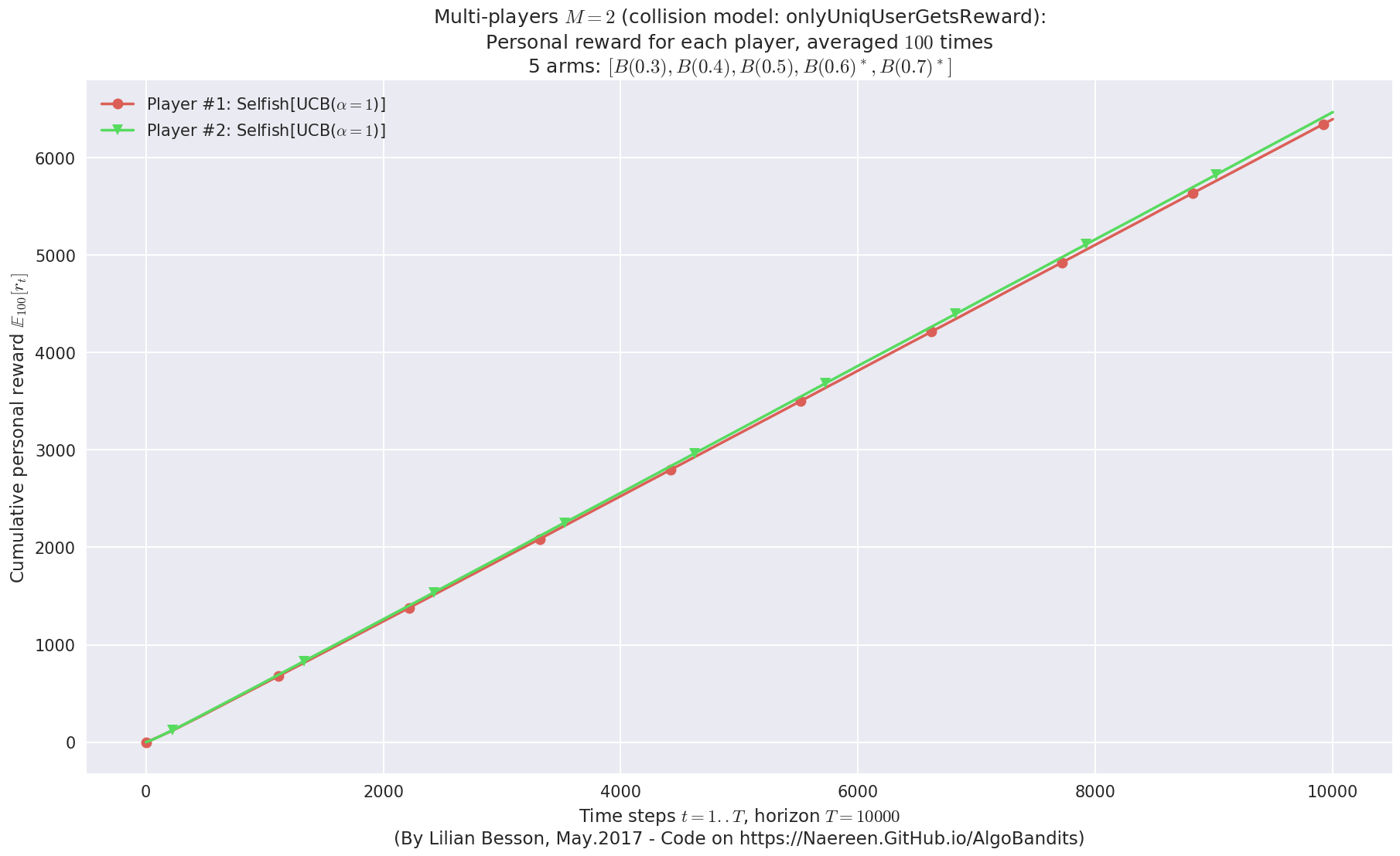
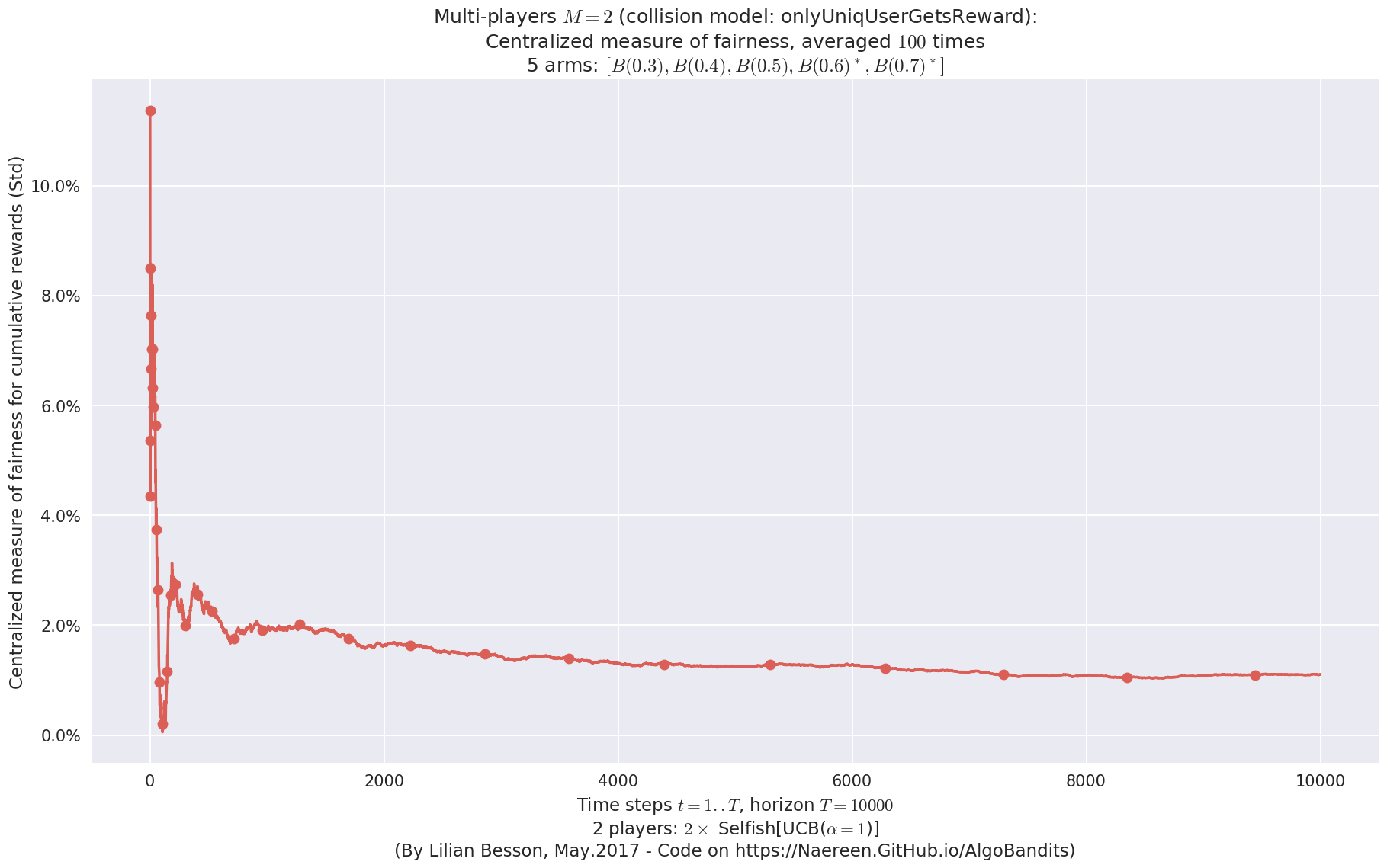
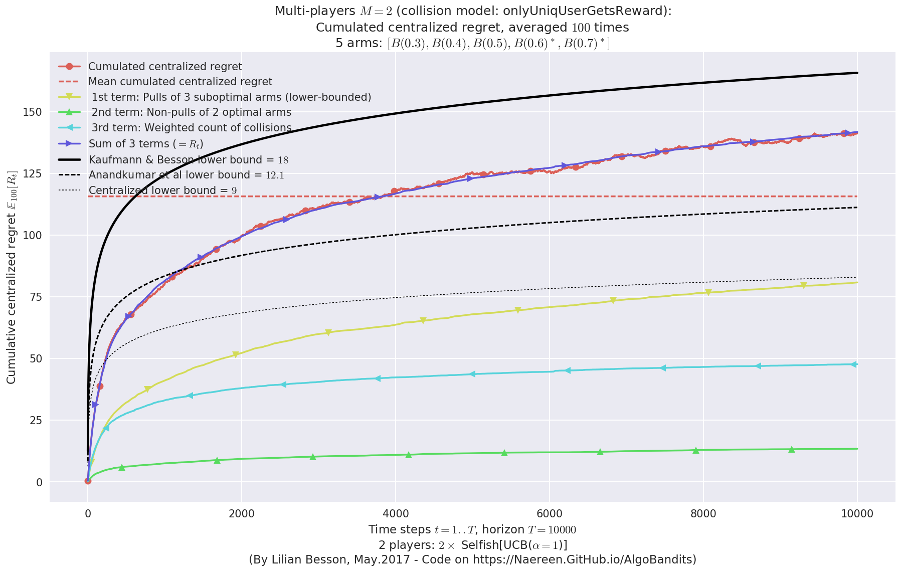
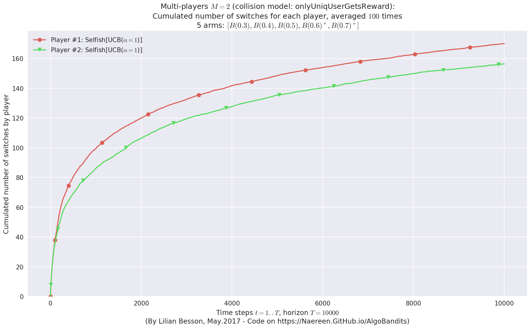
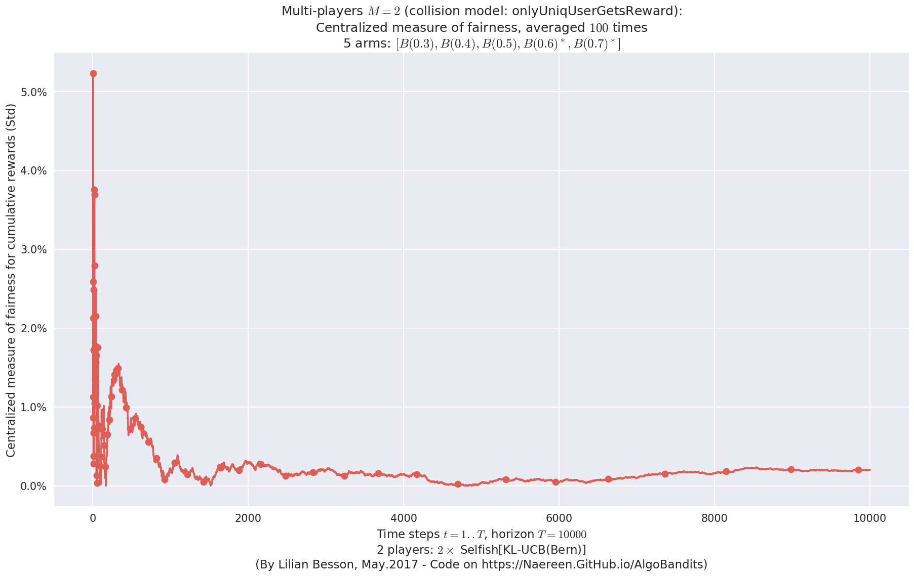
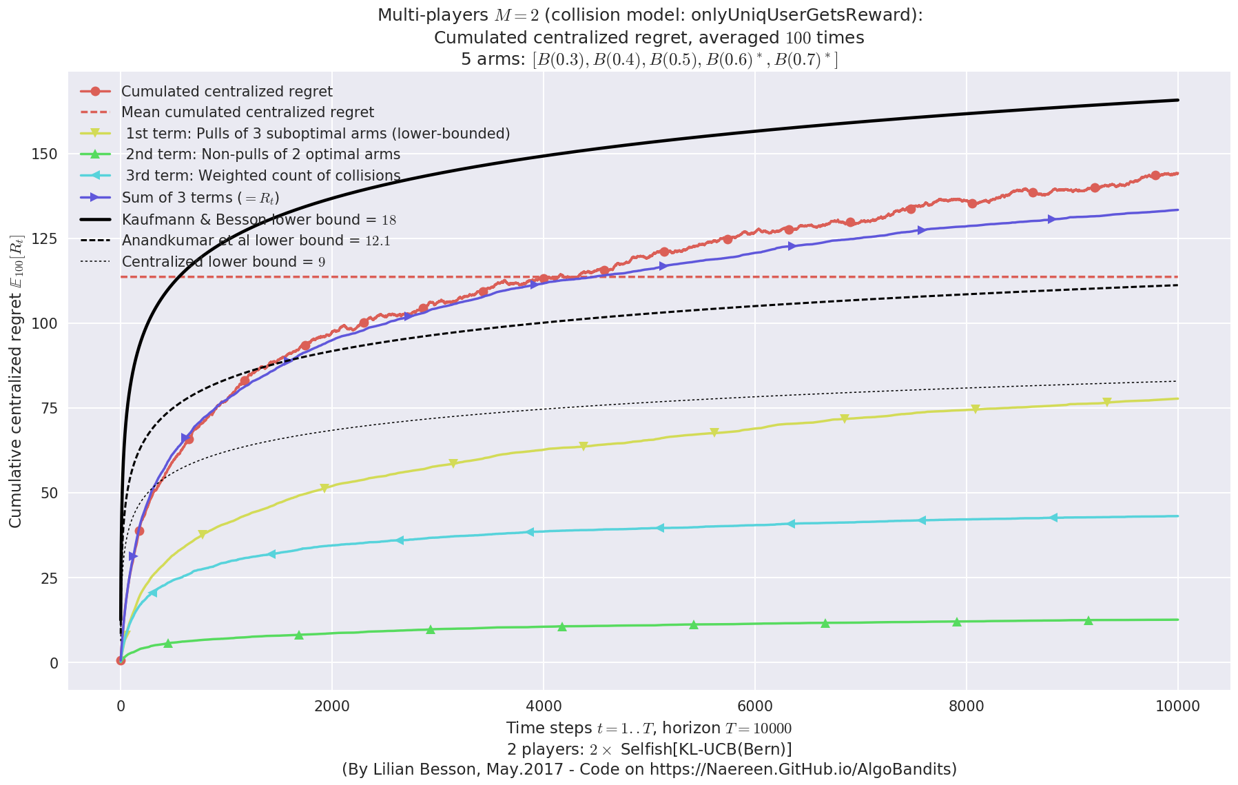
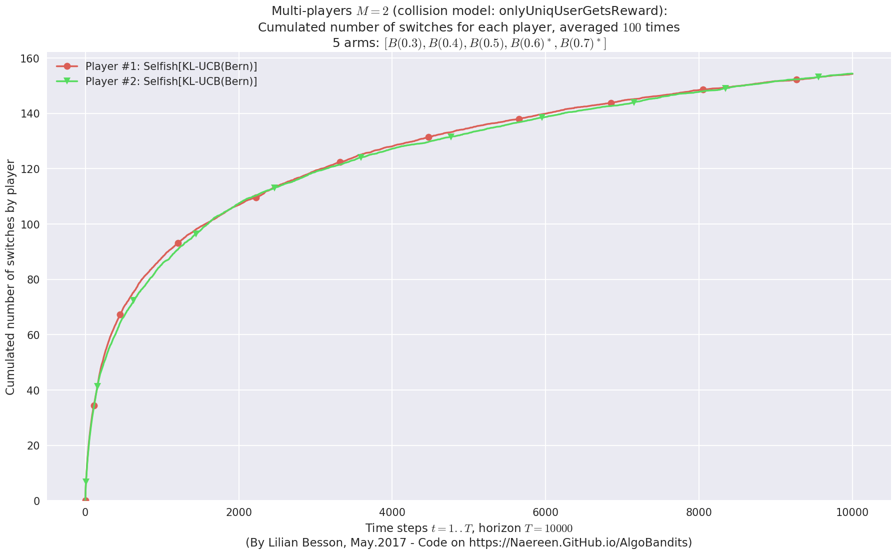
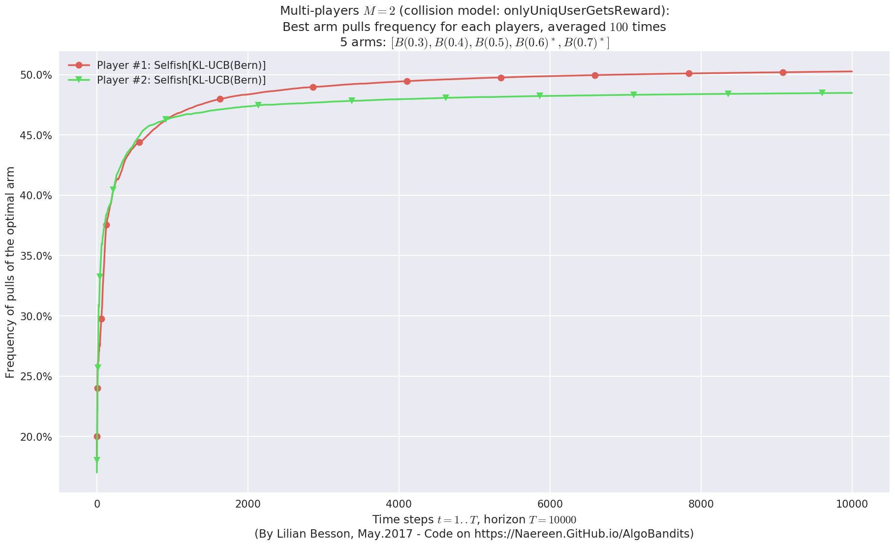
\(\mu = [0.3, 0.4, 0.5, 0.6, 0.7]\) was an easy Bernoulli problem.
In [25]:
for playersId in tqdm(range(len(evs)), desc="Policies"):
    evaluation = evaluators[0][playersId]
    plotAll(evaluation, 0)
Final ranking for this environment #0 :
- Player #2, '#2<$\rho^{\mathrm{Rand}}$[UCB($\alpha=1$)]>'        was ranked      1 / 2 for this simulation (last rewards = 6402.04).
- Player #1, '#1<$\rho^{\mathrm{Rand}}$[UCB($\alpha=1$)]>'        was ranked      2 / 2 for this simulation (last rewards = 6335.19).
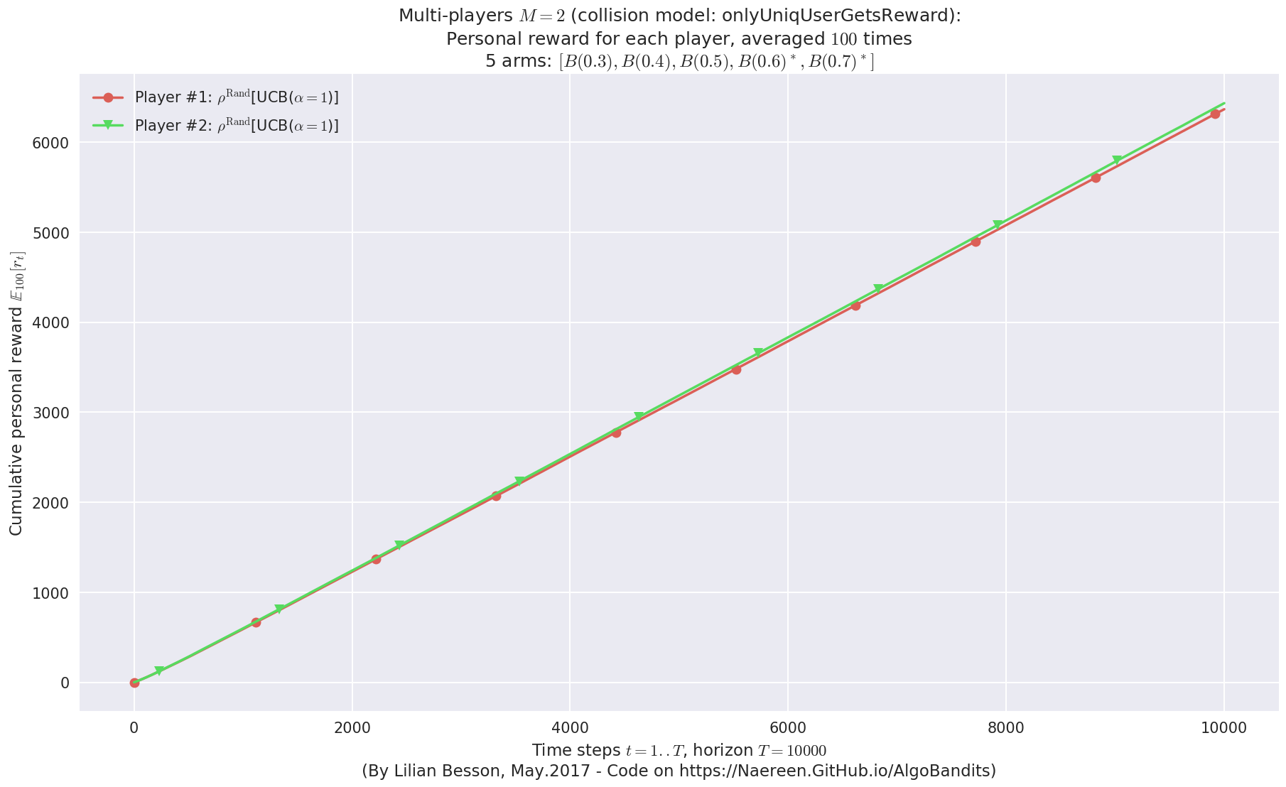
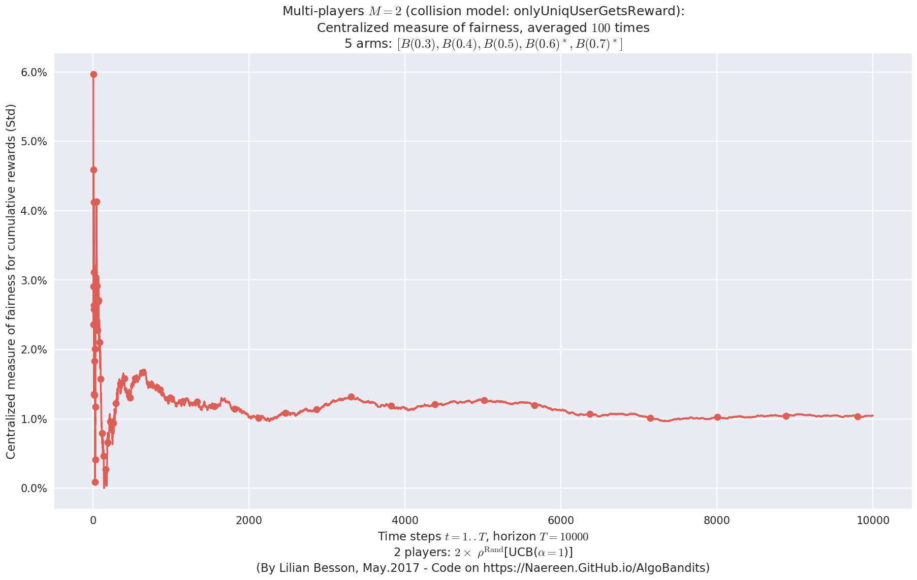
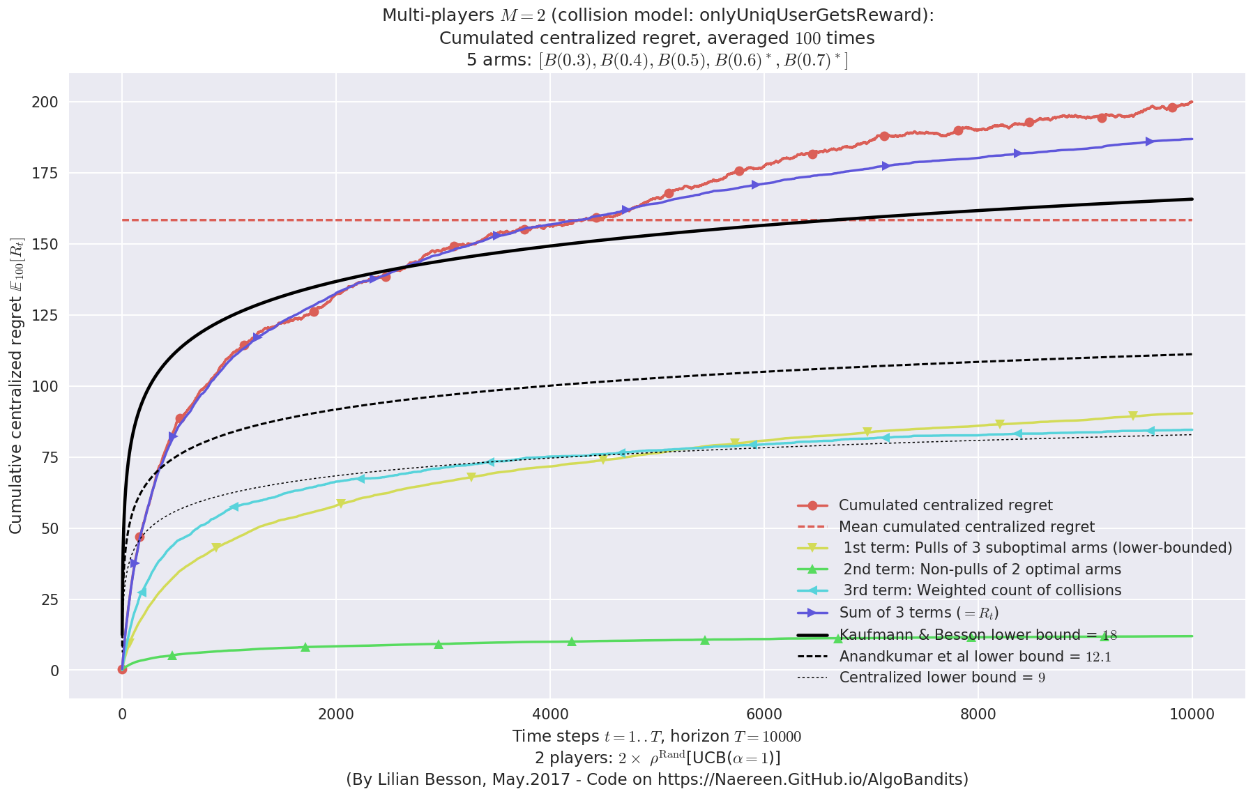
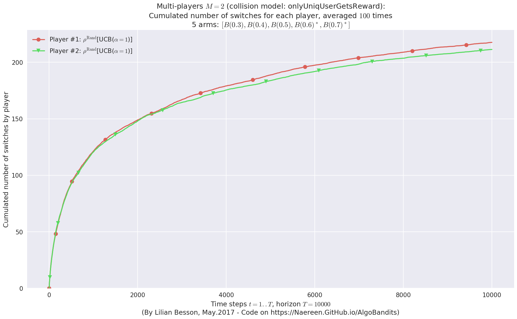
 -  For 2 players, Anandtharam et al. centralized lower-bound gave = 9 ...
 -  For 2 players, our lower bound gave = 18 ...
 -  For 2 players, the initial lower bound in Theorem 6 from [Anandkumar et al., 2010] gave = 12.1 ...

This MAB problem has:
 - a [Lai & Robbins] complexity constant C(mu) = 9.46 for 1-player problem ...
 - a Optimal Arm Identification factor H_OI(mu) = 60.00% ...
 - [Anandtharam et al] centralized lowerbound = 18,
 - Our decentralized lowerbound = 12.1,
 - [Anandkumar et al] decentralized lowerbound = 9
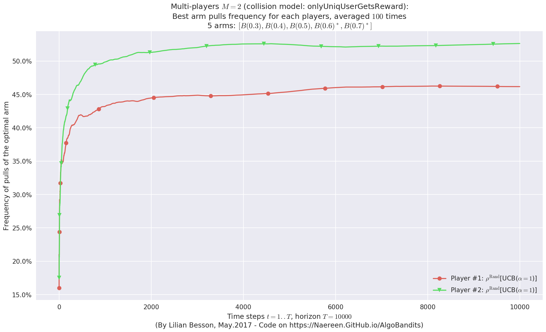
No upper bound for the non-cumulated number of collisions...
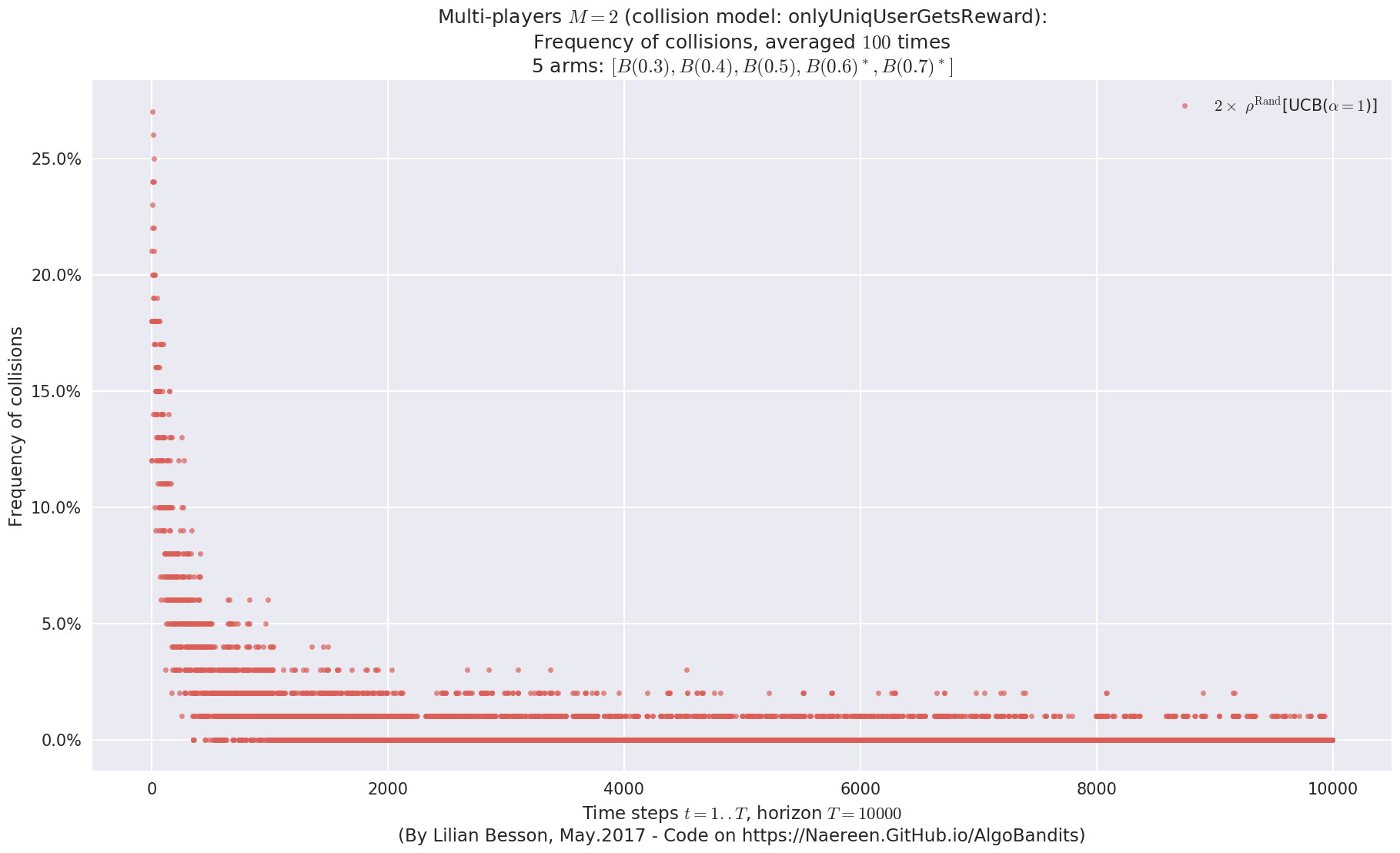
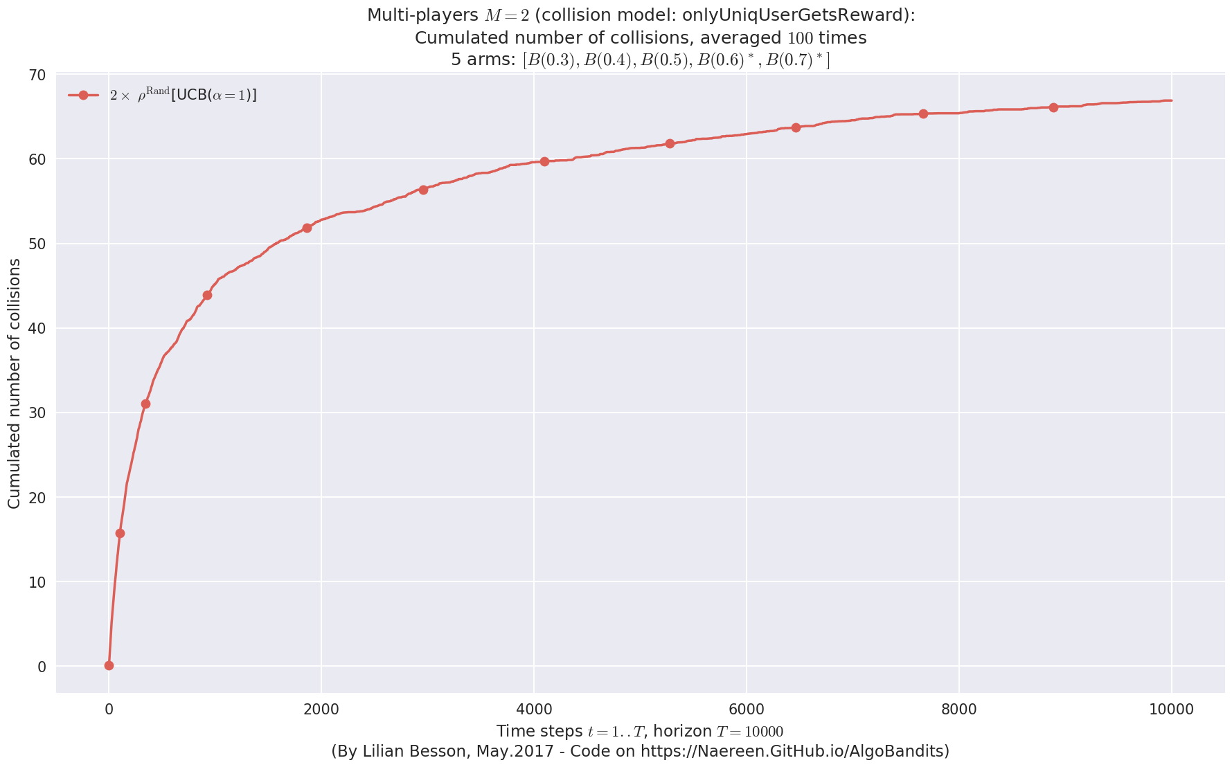
No upper bound for the non-cumulated number of collisions...
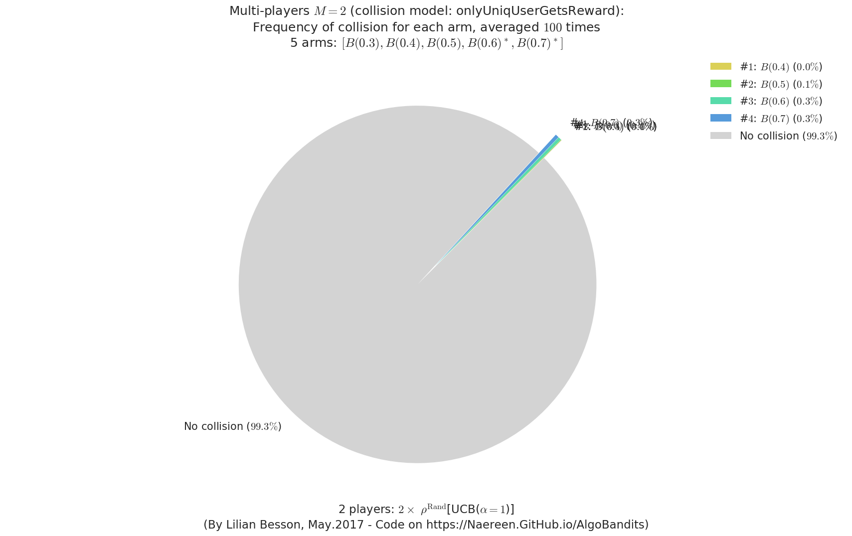
  - For #$0$: $B(0.3)$ ($0.0%$$\%$),    frequency of collisions is 8.4e-05  ...
  - For #$1$: $B(0.4)$ ($0.0%$$\%$),    frequency of collisions is 0.000192  ...
  - For #$2$: $B(0.5)$ ($0.1%$$\%$),    frequency of collisions is 0.0005  ...
  - For #$3$: $B(0.6)$ ($0.3%$$\%$),    frequency of collisions is 0.002623  ...
  - For #$4$: $B(0.7)$ ($0.3%$$\%$),    frequency of collisions is 0.003291  ...
Final ranking for this environment #0 :
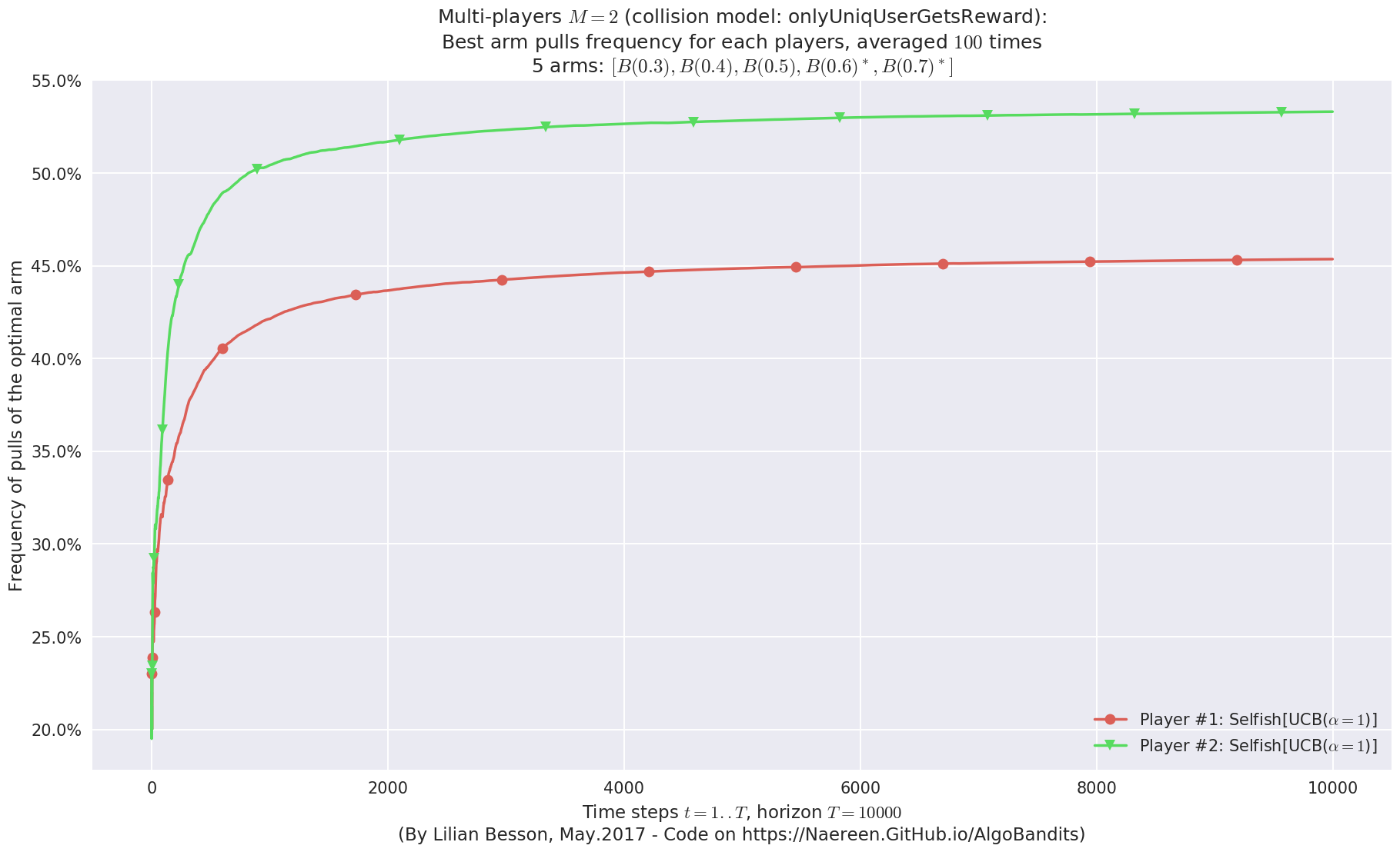
- Player #2, '#2<Selfish[UCB($\alpha=1$)]>'       was ranked      1 / 2 for this simulation (last rewards = 6433.37).
- Player #1, '#1<Selfish[UCB($\alpha=1$)]>'       was ranked      2 / 2 for this simulation (last rewards = 6362.26).
 -  For 2 players, Anandtharam et al. centralized lower-bound gave = 9 ...
 -  For 2 players, our lower bound gave = 18 ...
 -  For 2 players, the initial lower bound in Theorem 6 from [Anandkumar et al., 2010] gave = 12.1 ...

This MAB problem has:
 - a [Lai & Robbins] complexity constant C(mu) = 9.46 for 1-player problem ...
 - a Optimal Arm Identification factor H_OI(mu) = 60.00% ...
 - [Anandtharam et al] centralized lowerbound = 18,
 - Our decentralized lowerbound = 12.1,
 - [Anandkumar et al] decentralized lowerbound = 9
No upper bound for the non-cumulated number of collisions...
No upper bound for the non-cumulated number of collisions...

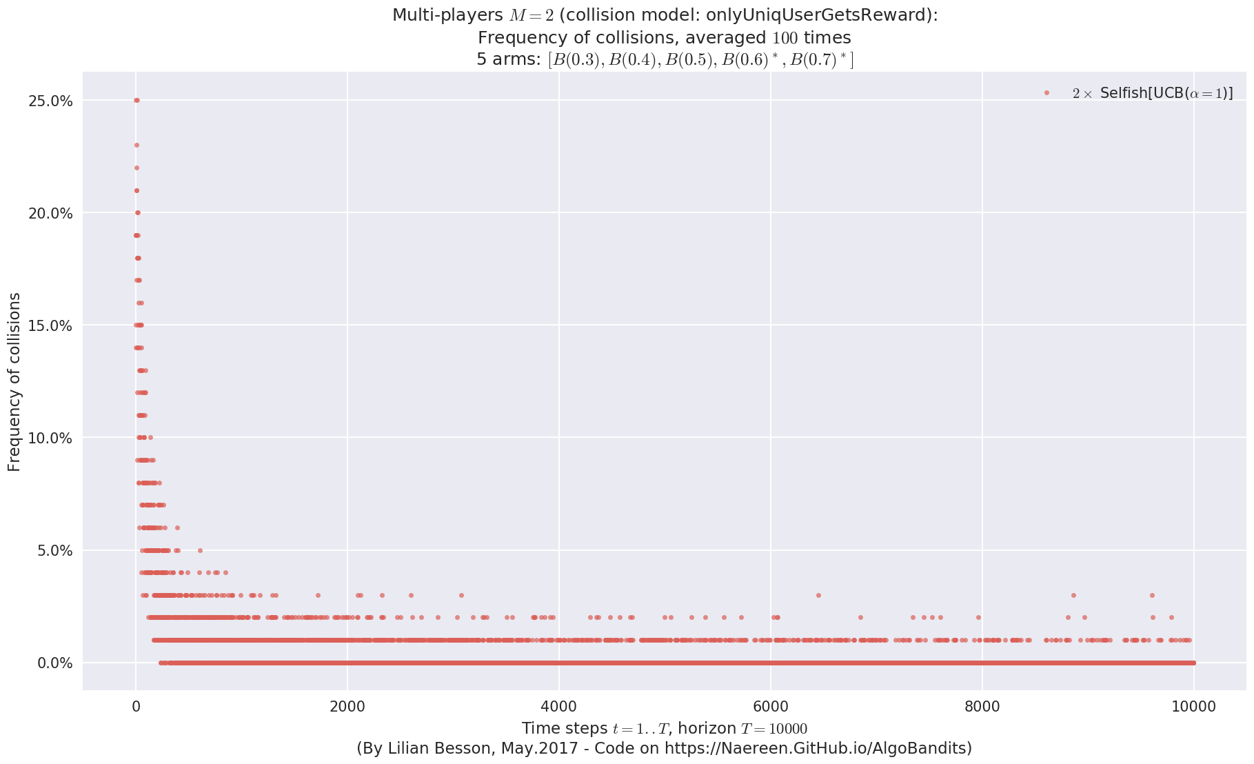
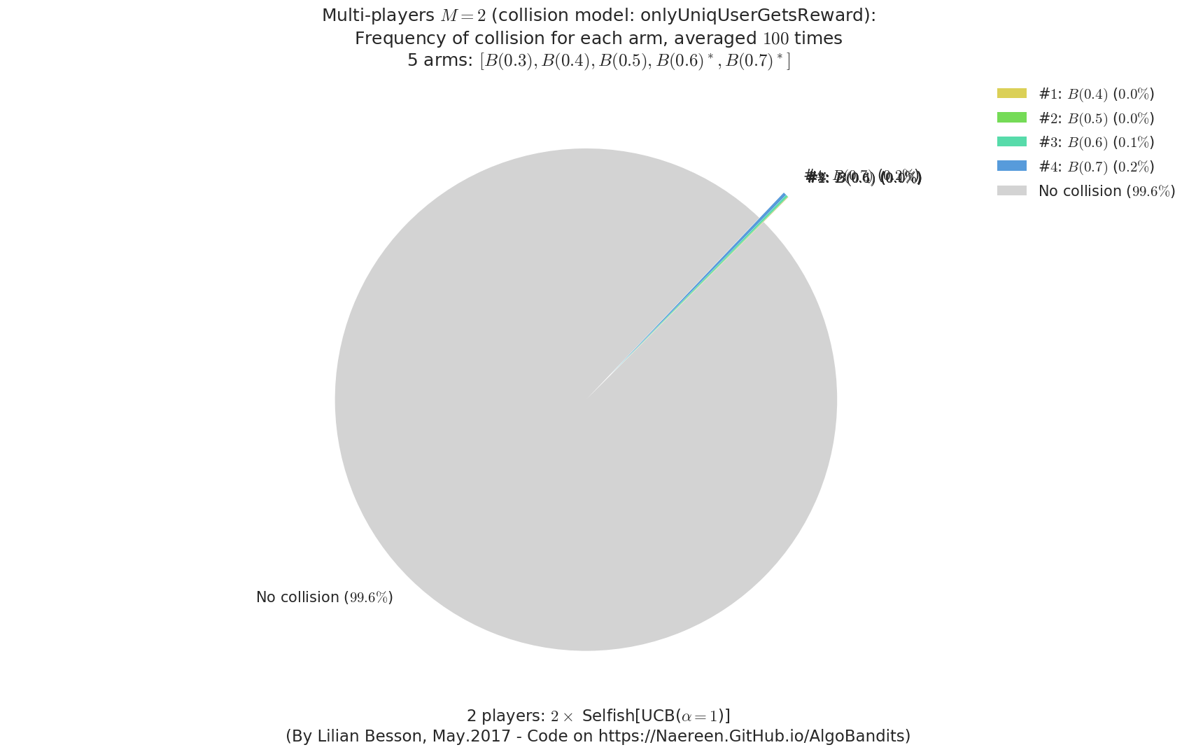
  - For #$0$: $B(0.3)$ ($0.0%$$\%$),    frequency of collisions is 8.7e-05  ...
  - For #$1$: $B(0.4)$ ($0.0%$$\%$),    frequency of collisions is 0.000167  ...
  - For #$2$: $B(0.5)$ ($0.0%$$\%$),    frequency of collisions is 0.000356  ...
  - For #$3$: $B(0.6)$ ($0.1%$$\%$),    frequency of collisions is 0.001135  ...
  - For #$4$: $B(0.7)$ ($0.2%$$\%$),    frequency of collisions is 0.002043  ...
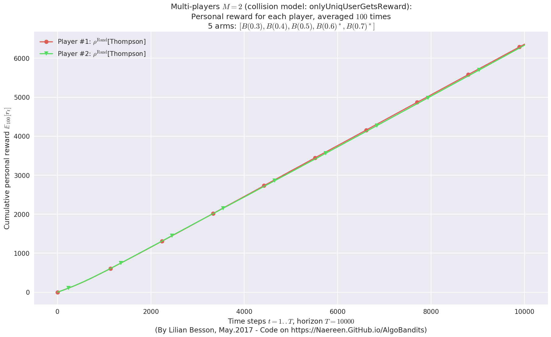
Final ranking for this environment #0 :
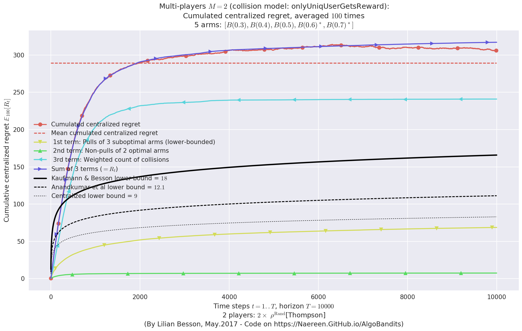
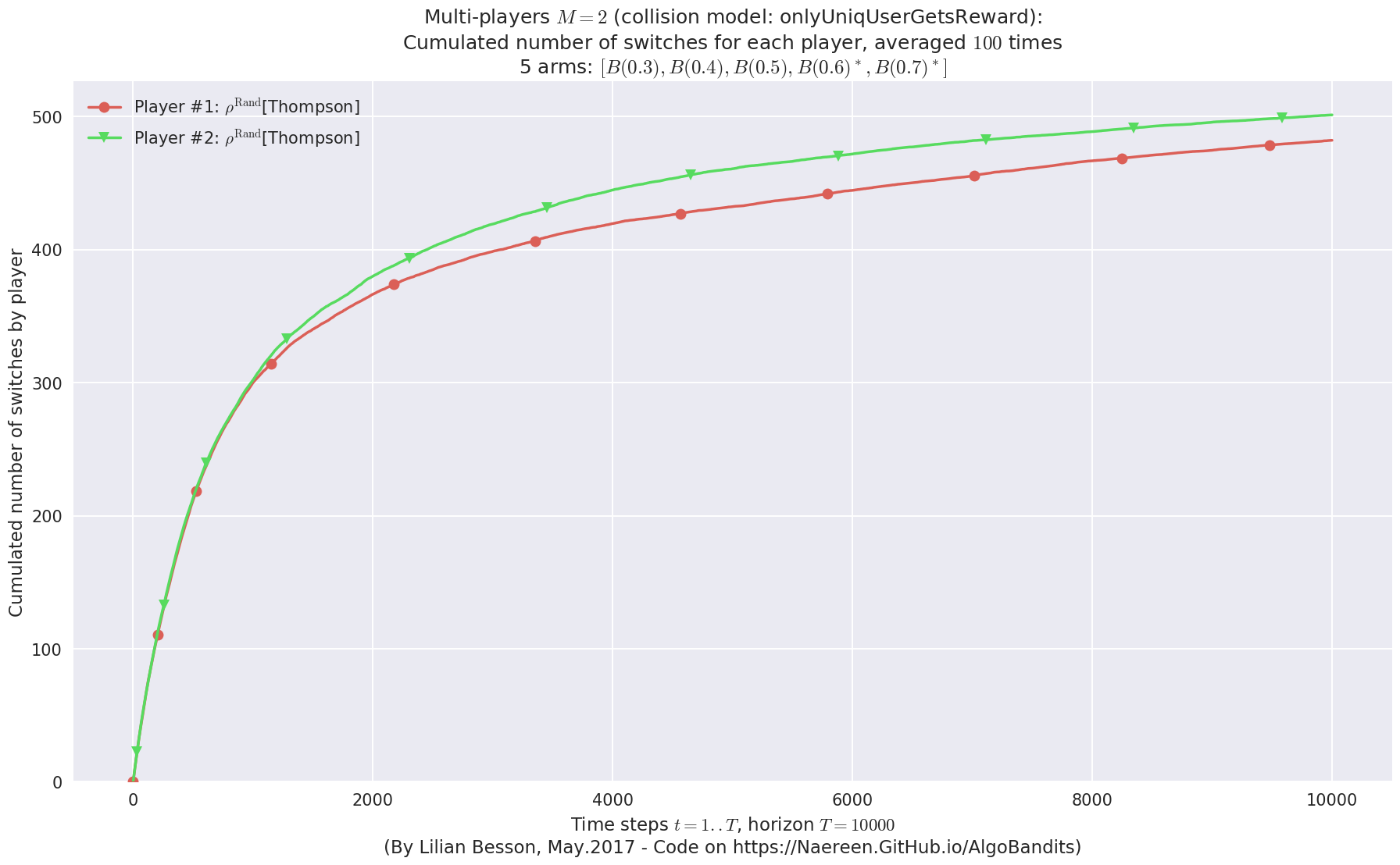
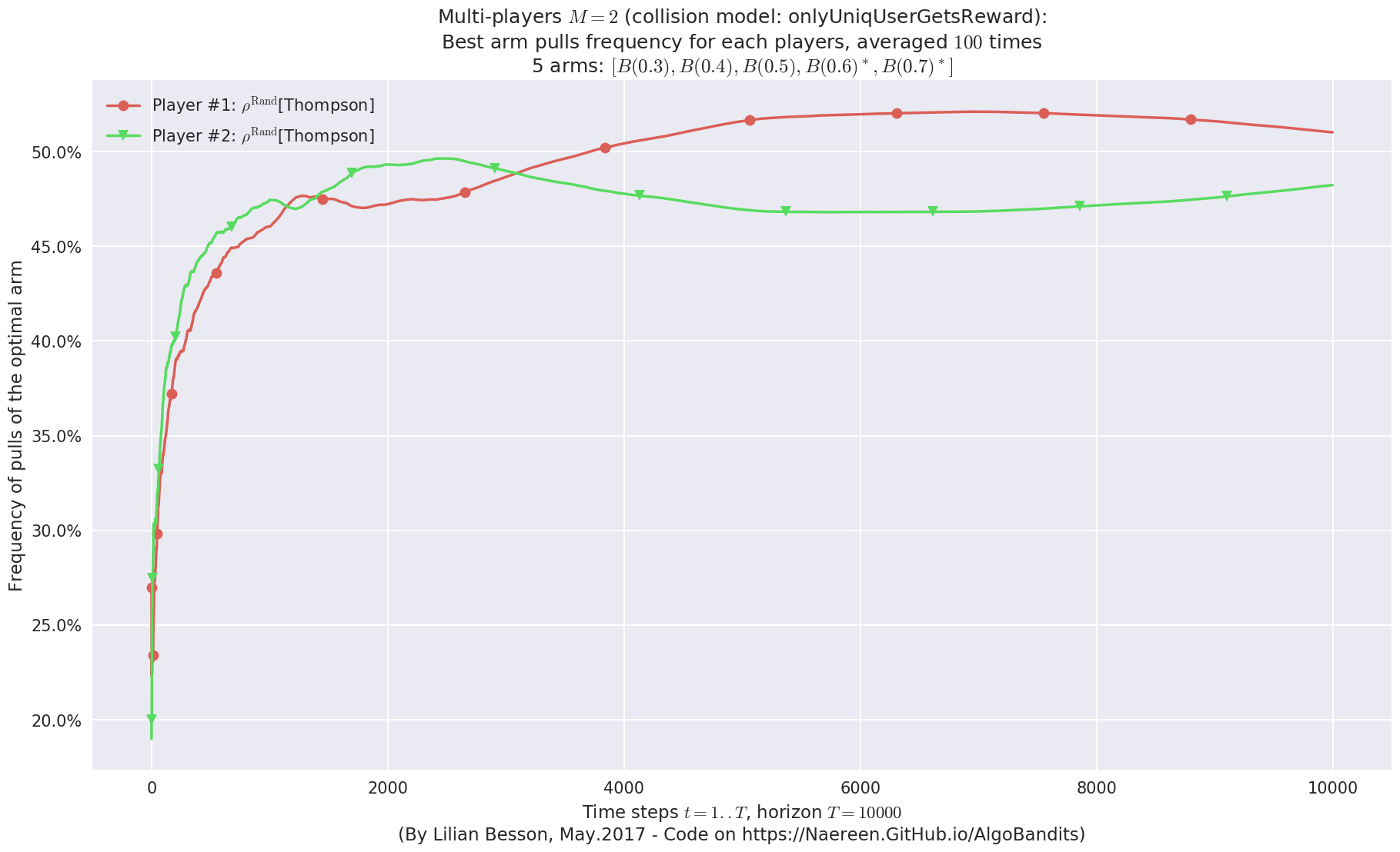
- Player #1, '#1<$\rho^{\mathrm{Rand}}$[Thompson]>'       was ranked      1 / 2 for this simulation (last rewards = 6328.66).
- Player #2, '#2<$\rho^{\mathrm{Rand}}$[Thompson]>'       was ranked      2 / 2 for this simulation (last rewards = 6301.73).
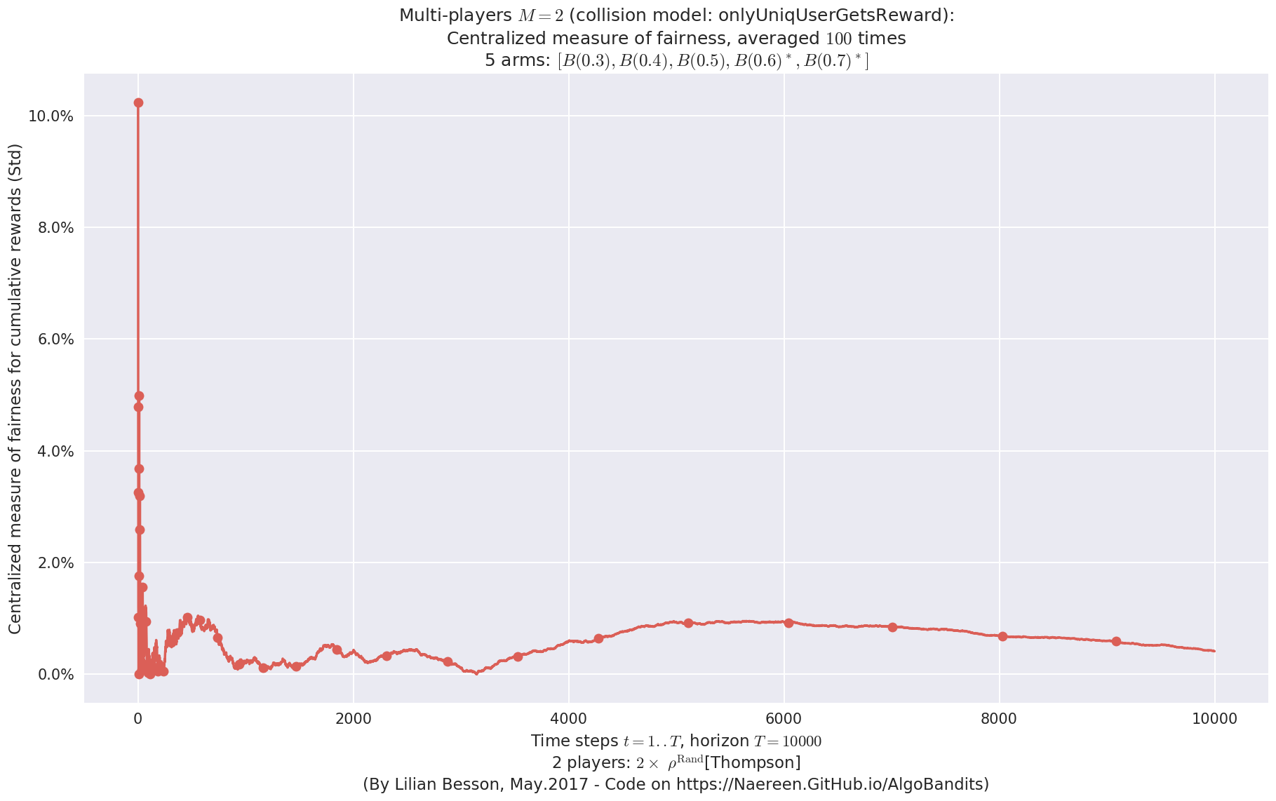
 -  For 2 players, Anandtharam et al. centralized lower-bound gave = 9 ...
 -  For 2 players, our lower bound gave = 18 ...
 -  For 2 players, the initial lower bound in Theorem 6 from [Anandkumar et al., 2010] gave = 12.1 ...

This MAB problem has:
 - a [Lai & Robbins] complexity constant C(mu) = 9.46 for 1-player problem ...
 - a Optimal Arm Identification factor H_OI(mu) = 60.00% ...
 - [Anandtharam et al] centralized lowerbound = 18,
 - Our decentralized lowerbound = 12.1,
 - [Anandkumar et al] decentralized lowerbound = 9
No upper bound for the non-cumulated number of collisions...
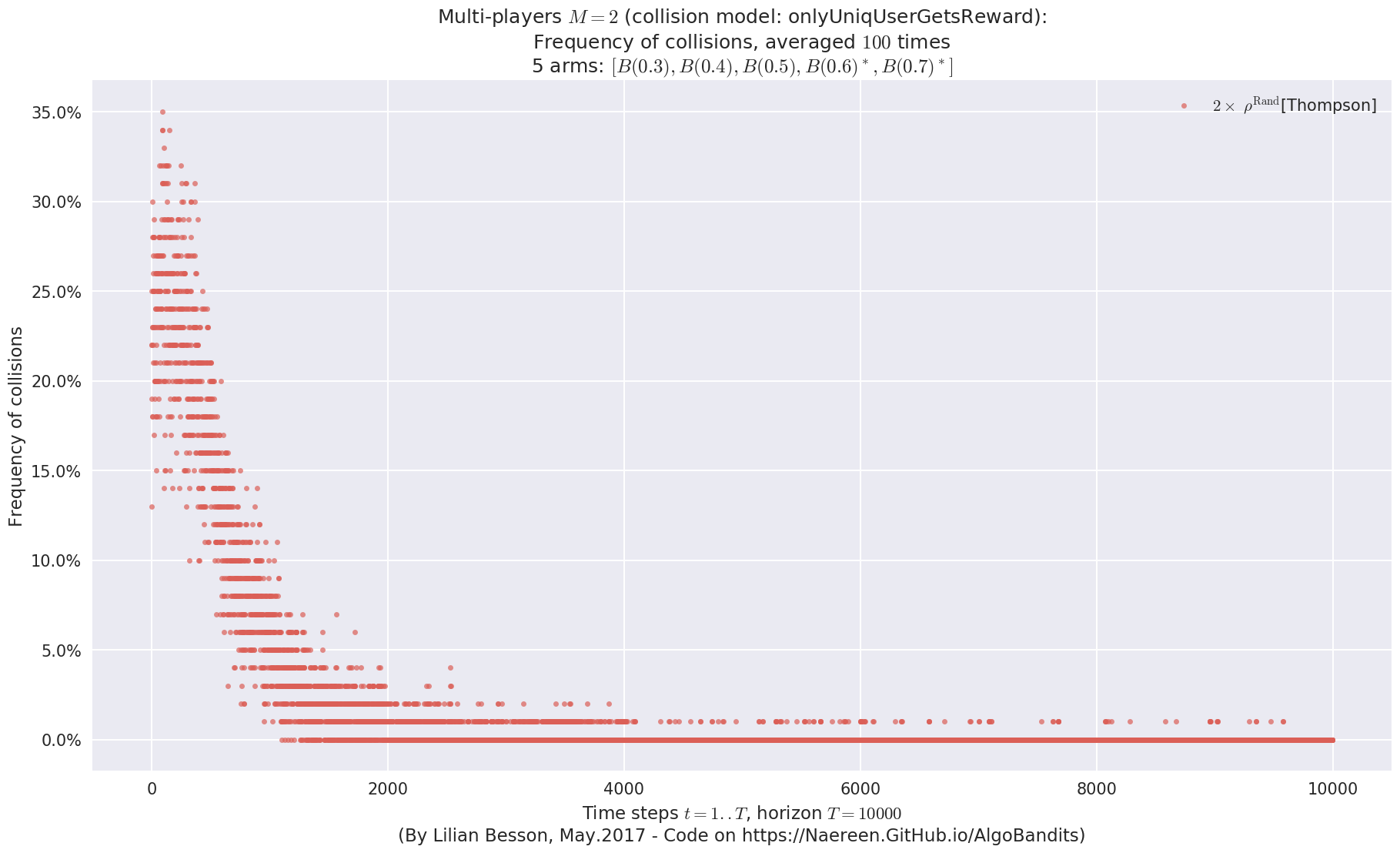
No upper bound for the non-cumulated number of collisions...
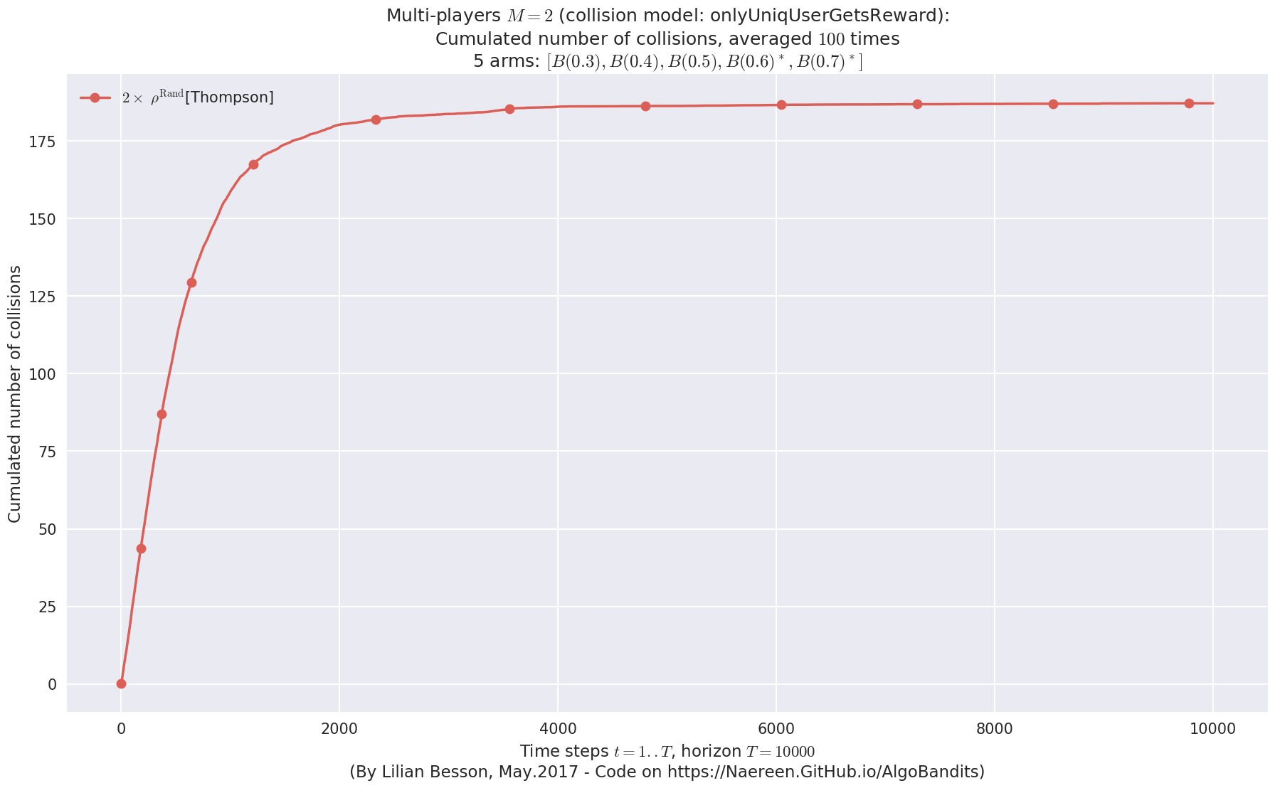
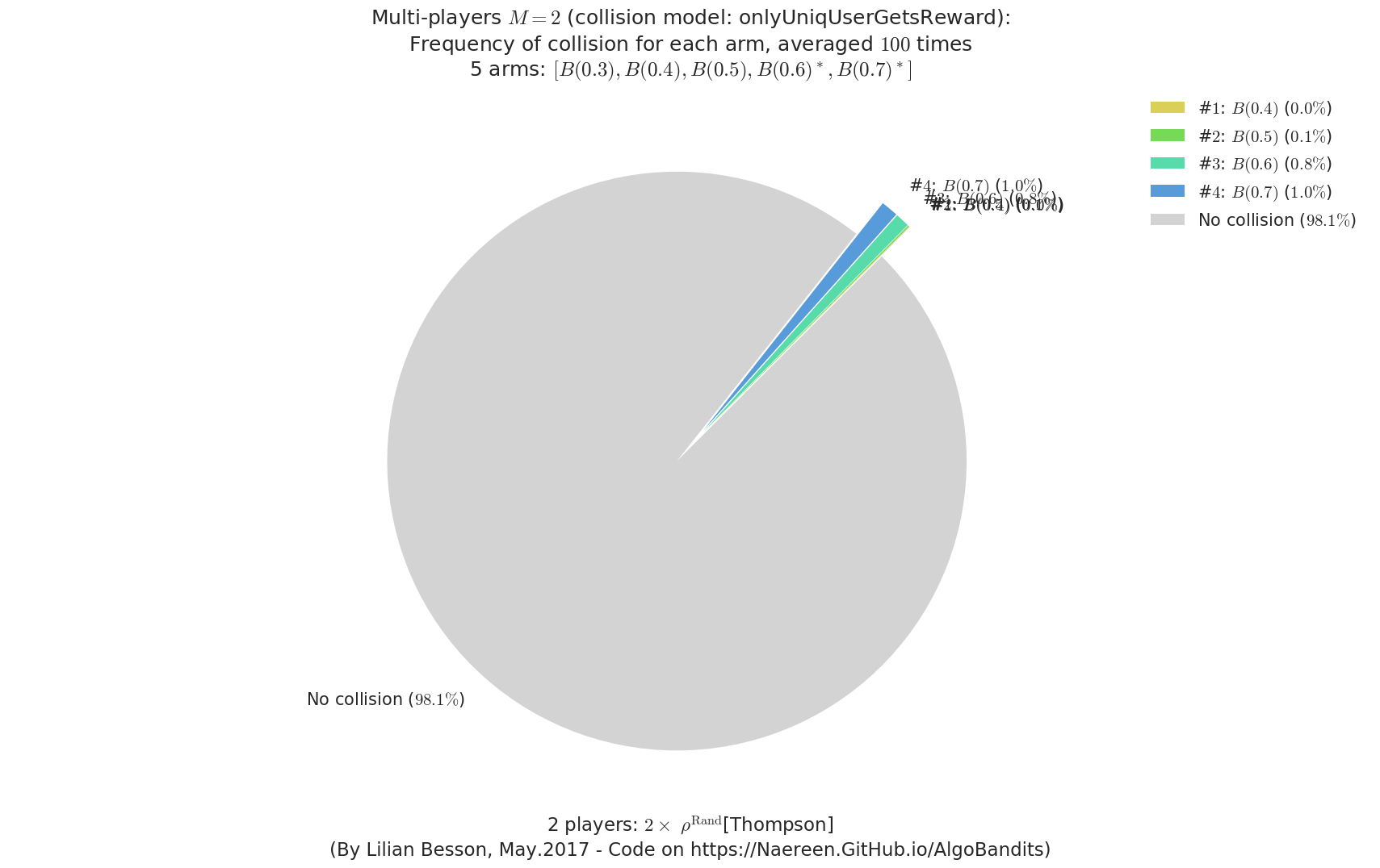
  - For #$0$: $B(0.3)$ ($0.0%$$\%$),    frequency of collisions is 9.7e-05  ...
  - For #$1$: $B(0.4)$ ($0.0%$$\%$),    frequency of collisions is 0.000257  ...
  - For #$2$: $B(0.5)$ ($0.1%$$\%$),    frequency of collisions is 0.000768  ...
  - For #$3$: $B(0.6)$ ($0.8%$$\%$),    frequency of collisions is 0.007895  ...
  - For #$4$: $B(0.7)$ ($1.0%$$\%$),    frequency of collisions is 0.009701  ...
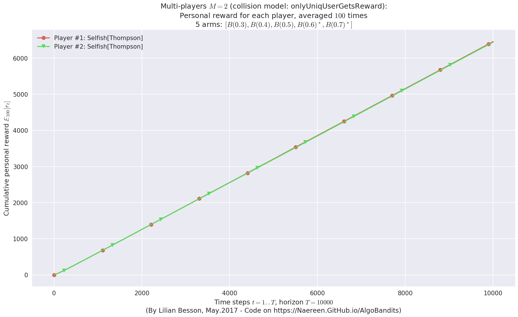
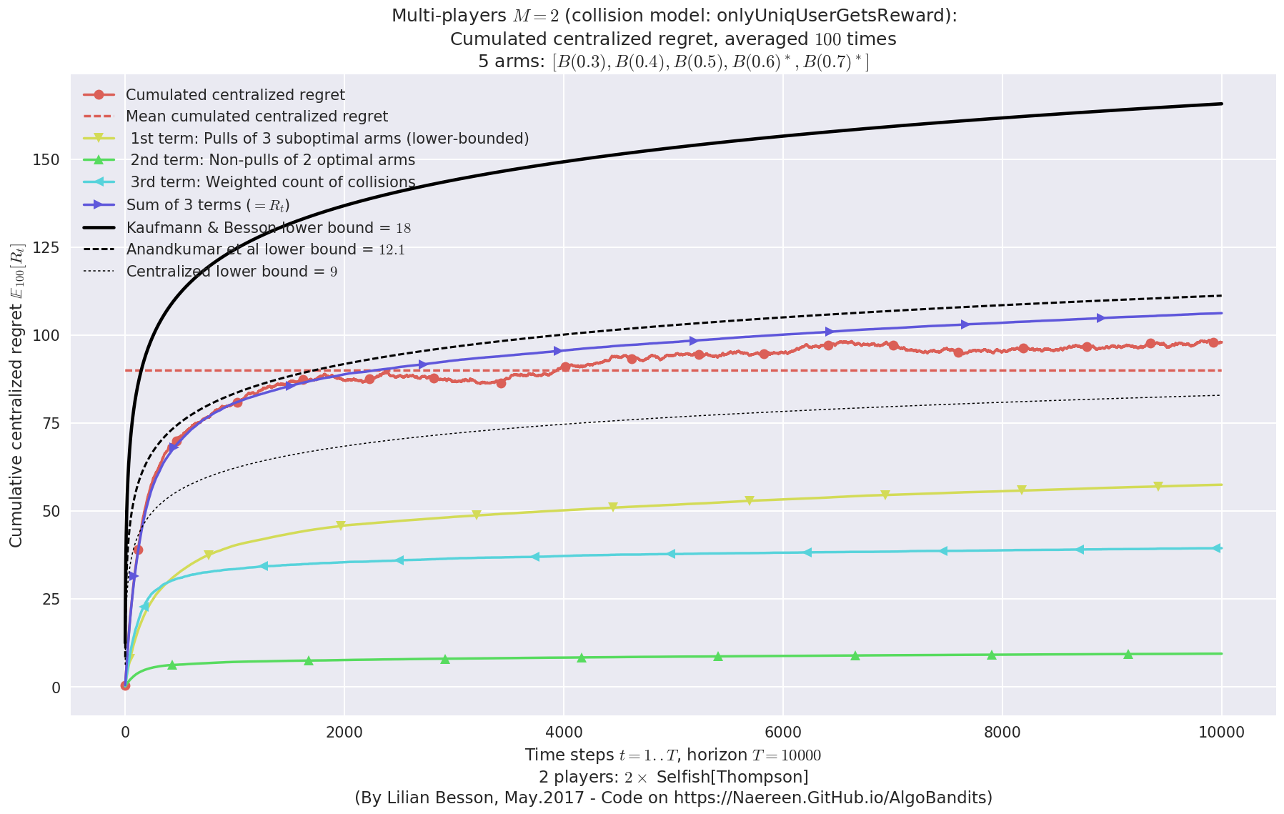
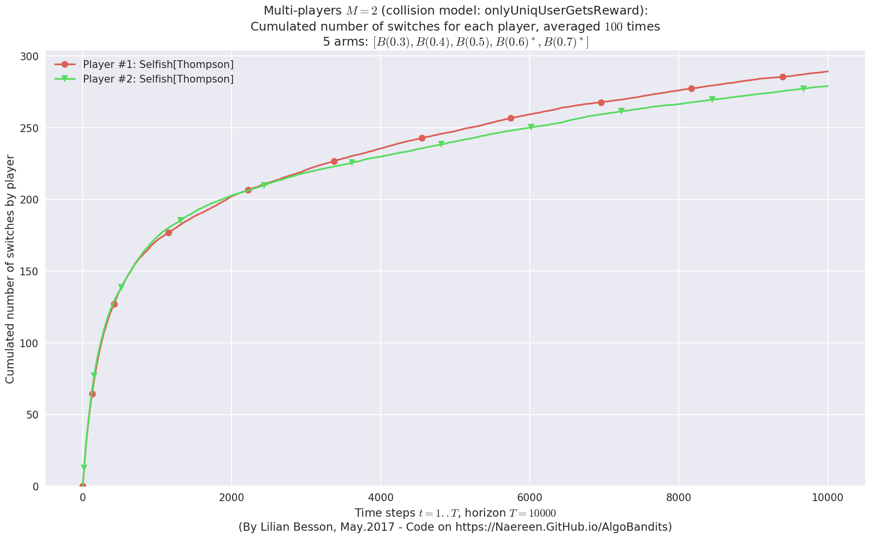
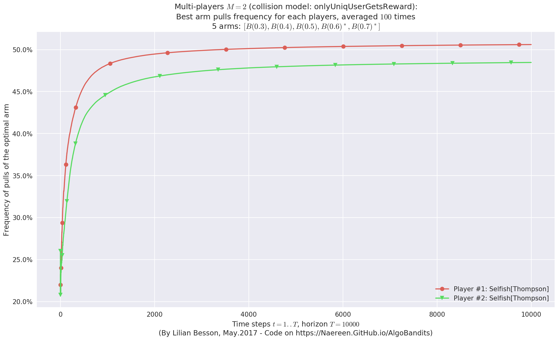
Final ranking for this environment #0 :
- Player #1, '#1<Selfish[Thompson]>'      was ranked      1 / 2 for this simulation (last rewards = 6427.68).
- Player #2, '#2<Selfish[Thompson]>'      was ranked      2 / 2 for this simulation (last rewards = 6410.71).
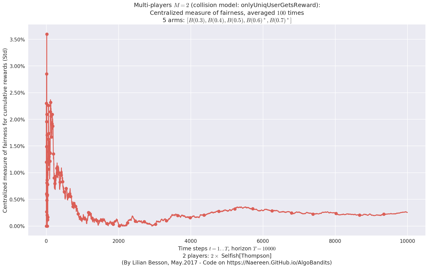
 -  For 2 players, Anandtharam et al. centralized lower-bound gave = 9 ...
 -  For 2 players, our lower bound gave = 18 ...
 -  For 2 players, the initial lower bound in Theorem 6 from [Anandkumar et al., 2010] gave = 12.1 ...

This MAB problem has:
 - a [Lai & Robbins] complexity constant C(mu) = 9.46 for 1-player problem ...
 - a Optimal Arm Identification factor H_OI(mu) = 60.00% ...
 - [Anandtharam et al] centralized lowerbound = 18,
 - Our decentralized lowerbound = 12.1,
 - [Anandkumar et al] decentralized lowerbound = 9
No upper bound for the non-cumulated number of collisions...
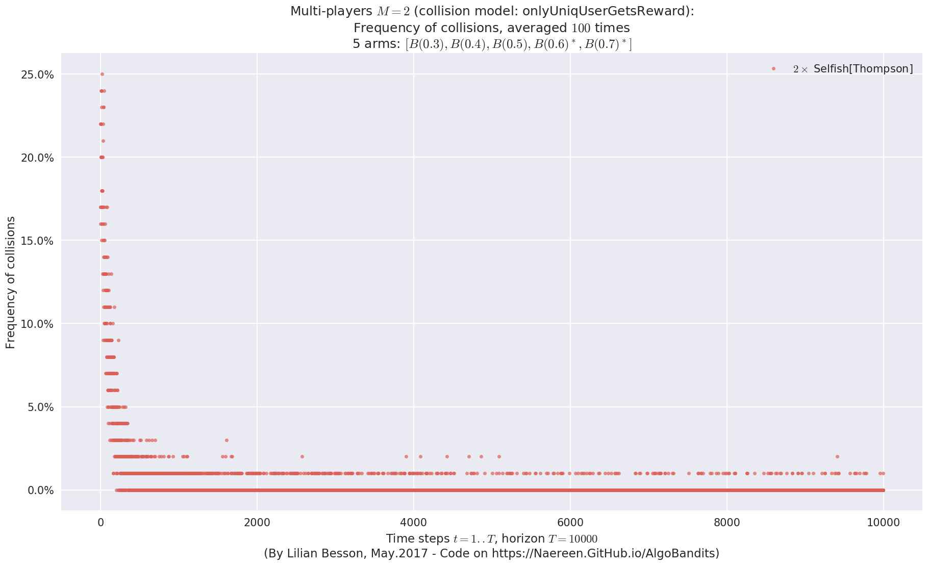
No upper bound for the non-cumulated number of collisions...
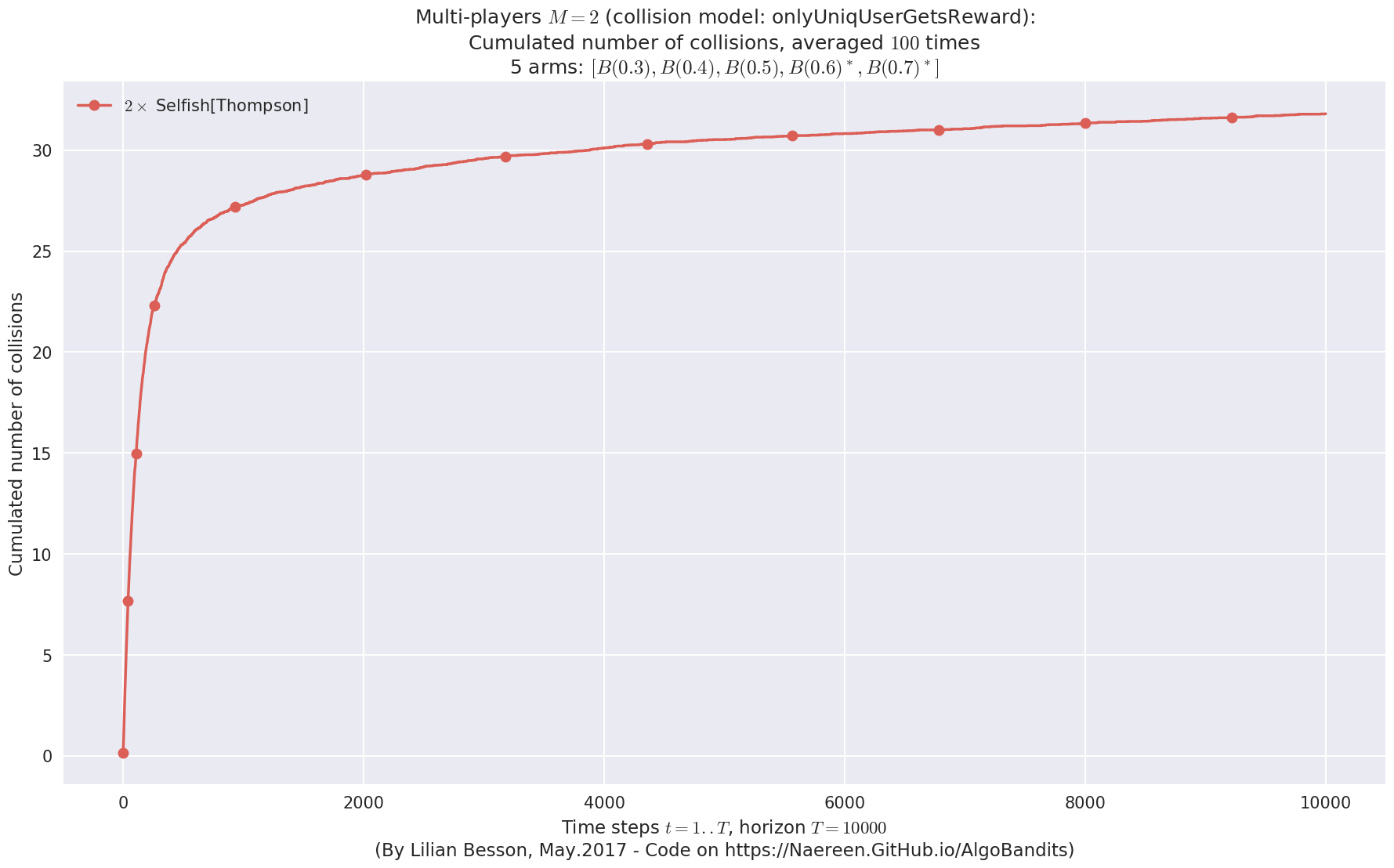
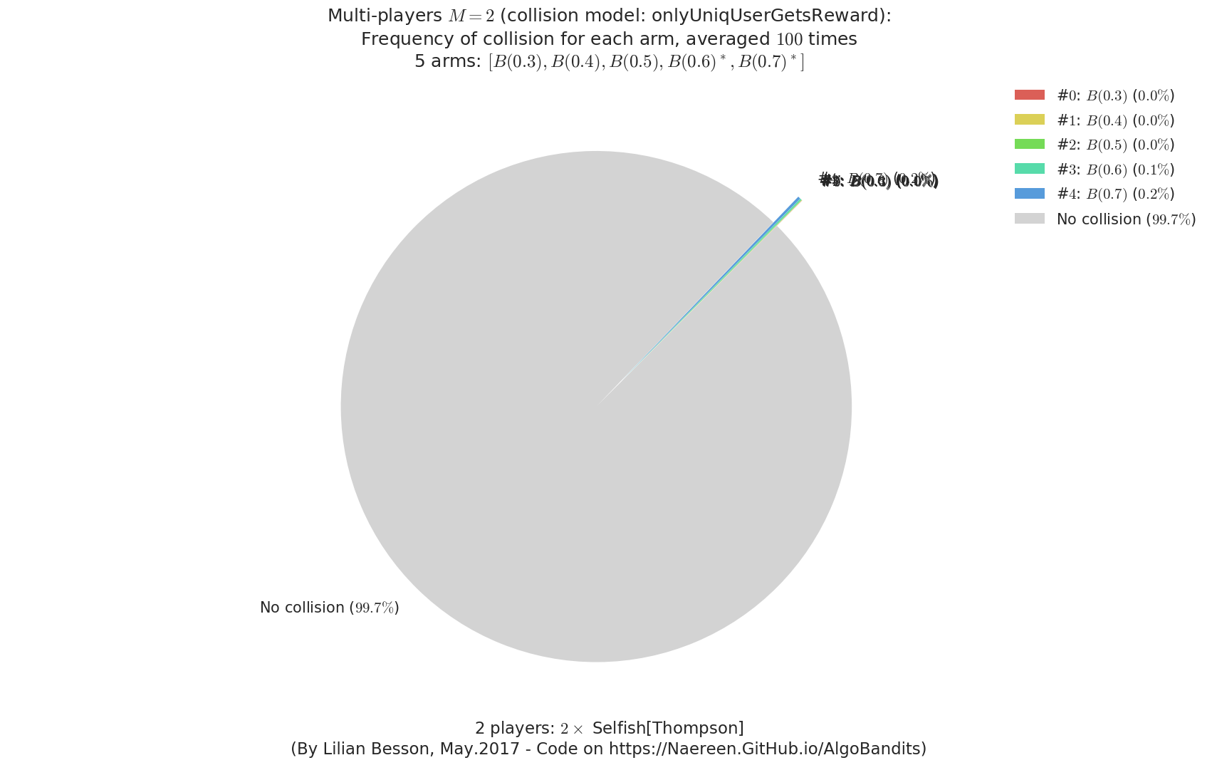
  - For #$0$: $B(0.3)$ ($0.0%$$\%$),    frequency of collisions is 0.000116  ...
  - For #$1$: $B(0.4)$ ($0.0%$$\%$),    frequency of collisions is 0.000194  ...
  - For #$2$: $B(0.5)$ ($0.0%$$\%$),    frequency of collisions is 0.000327  ...
  - For #$3$: $B(0.6)$ ($0.1%$$\%$),    frequency of collisions is 0.000871  ...
  - For #$4$: $B(0.7)$ ($0.2%$$\%$),    frequency of collisions is 0.001673  ...
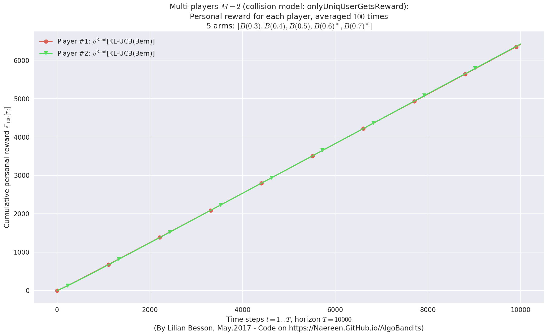
Final ranking for this environment #0 :
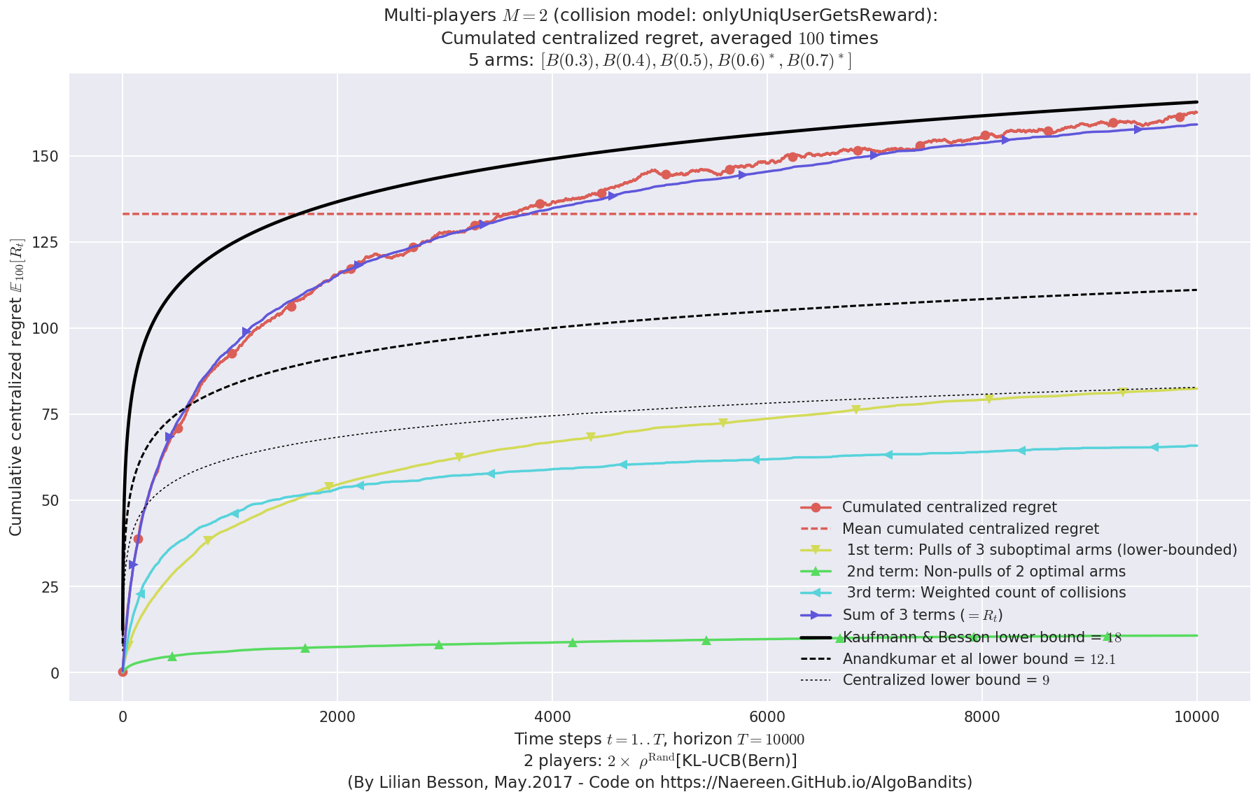
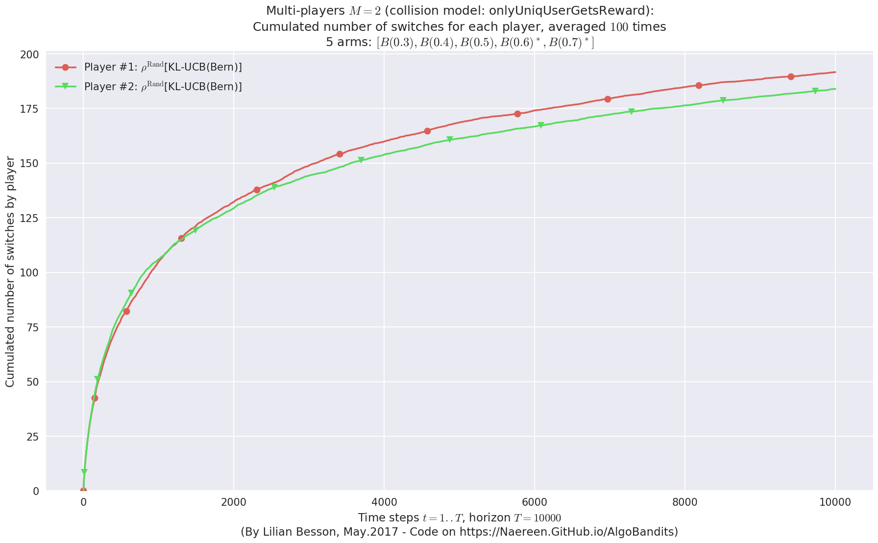
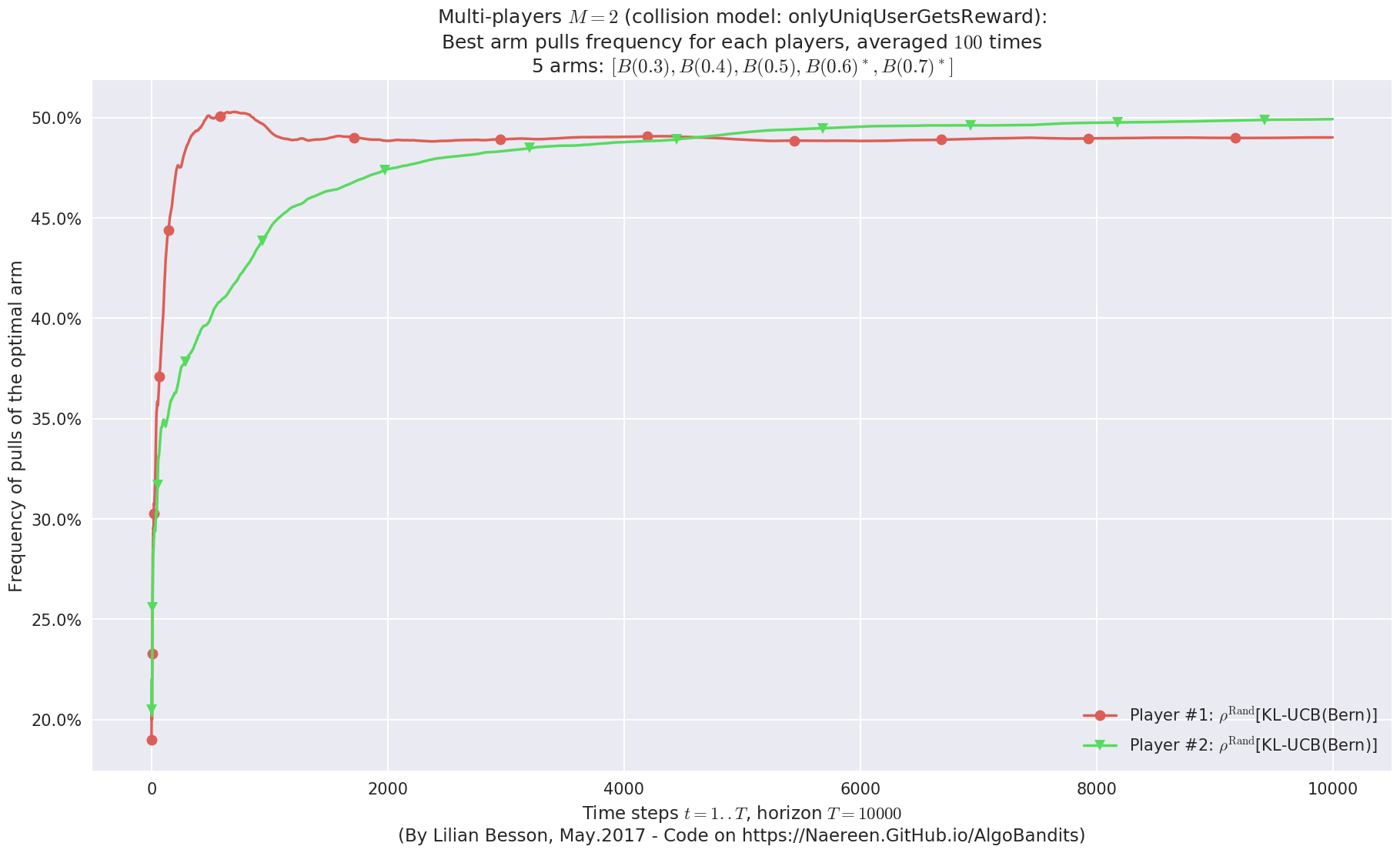
- Player #2, '#2<$\rho^{\mathrm{Rand}}$[KL-UCB(Bern)]>'   was ranked      1 / 2 for this simulation (last rewards = 6391.76).
- Player #1, '#1<$\rho^{\mathrm{Rand}}$[KL-UCB(Bern)]>'   was ranked      2 / 2 for this simulation (last rewards = 6381.88).
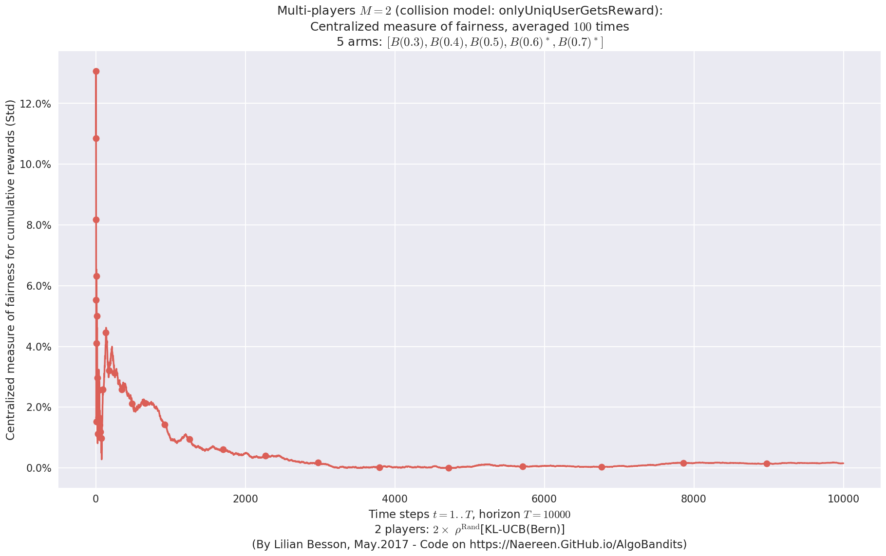
 -  For 2 players, Anandtharam et al. centralized lower-bound gave = 9 ...
 -  For 2 players, our lower bound gave = 18 ...
 -  For 2 players, the initial lower bound in Theorem 6 from [Anandkumar et al., 2010] gave = 12.1 ...

This MAB problem has:
 - a [Lai & Robbins] complexity constant C(mu) = 9.46 for 1-player problem ...
 - a Optimal Arm Identification factor H_OI(mu) = 60.00% ...
 - [Anandtharam et al] centralized lowerbound = 18,
 - Our decentralized lowerbound = 12.1,
 - [Anandkumar et al] decentralized lowerbound = 9
No upper bound for the non-cumulated number of collisions...
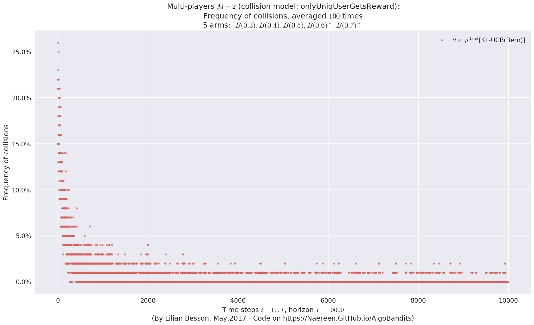
No upper bound for the non-cumulated number of collisions...
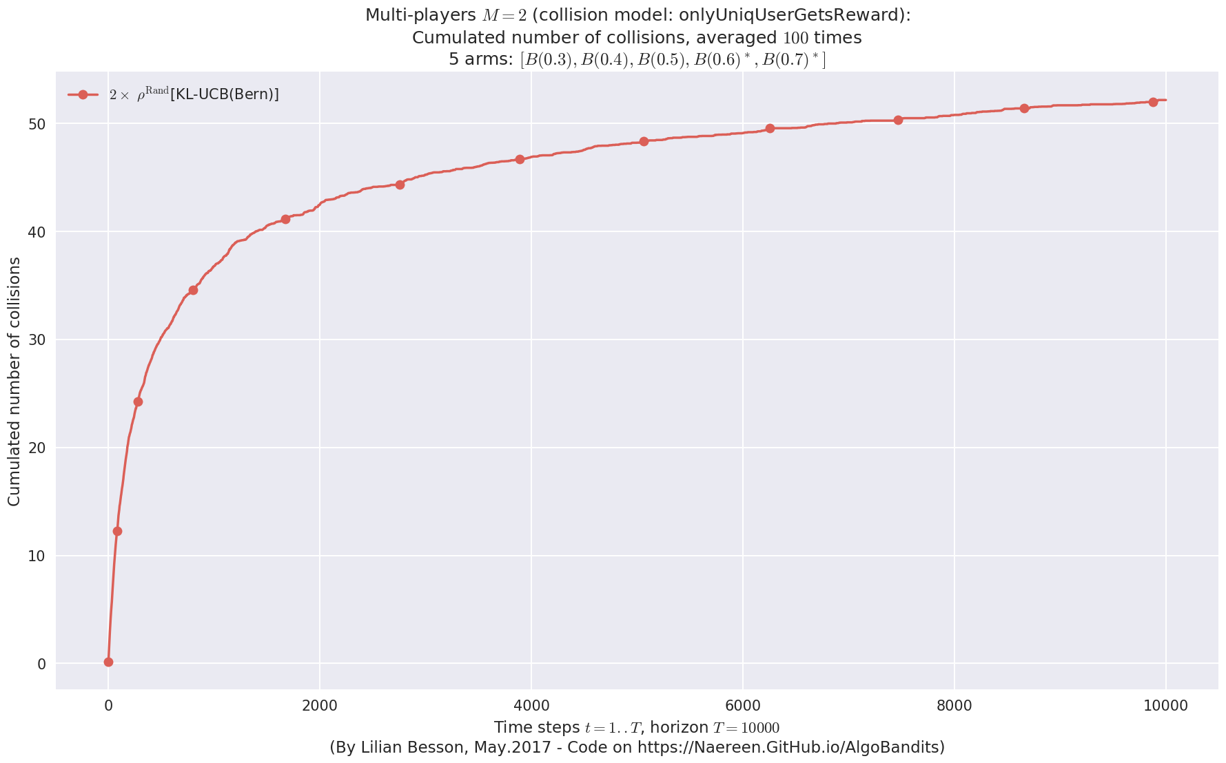
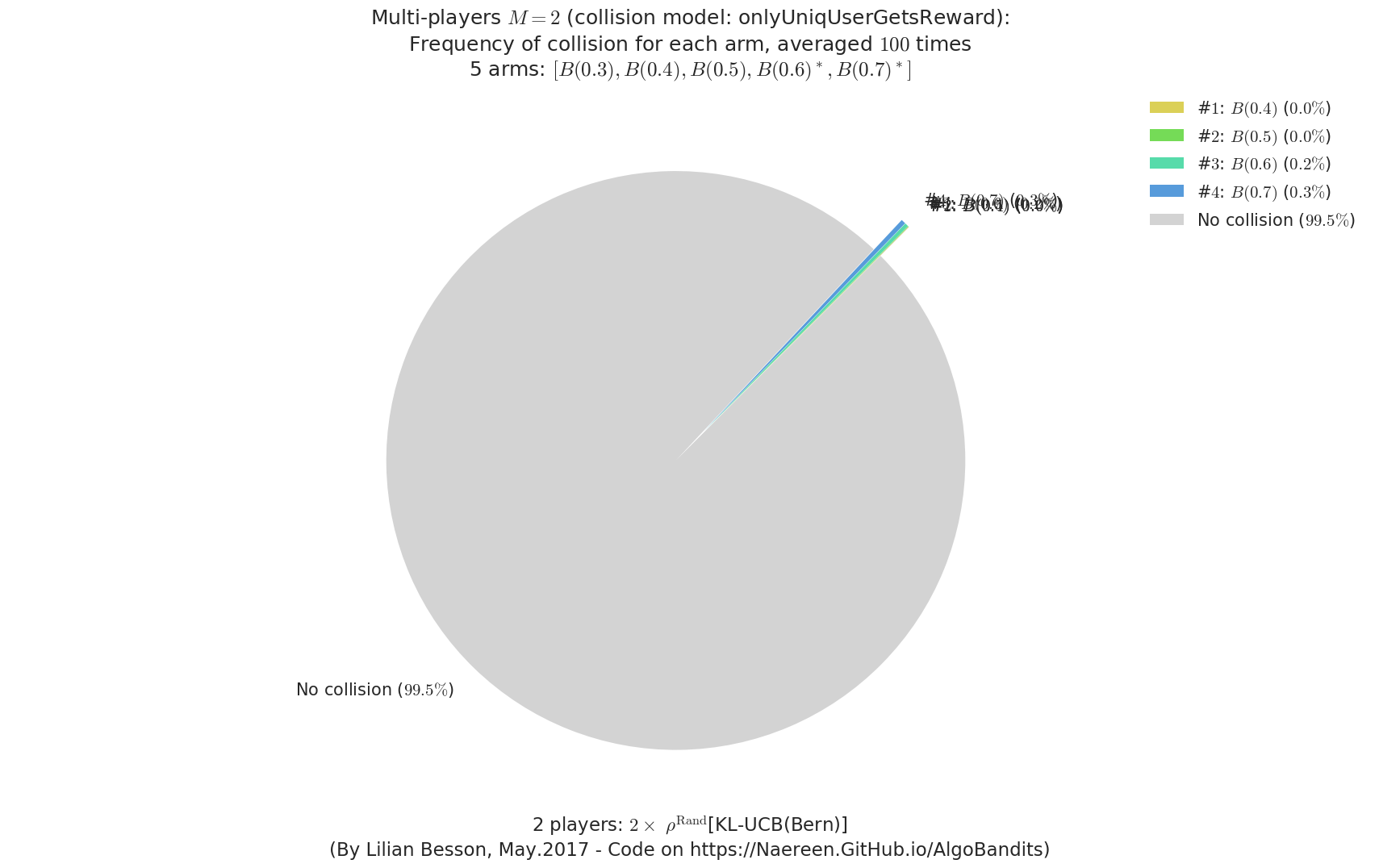
  - For #$0$: $B(0.3)$ ($0.0%$$\%$),    frequency of collisions is 8.8e-05  ...
  - For #$1$: $B(0.4)$ ($0.0%$$\%$),    frequency of collisions is 0.000153  ...
  - For #$2$: $B(0.5)$ ($0.0%$$\%$),    frequency of collisions is 0.000369  ...
  - For #$3$: $B(0.6)$ ($0.2%$$\%$),    frequency of collisions is 0.001991  ...
  - For #$4$: $B(0.7)$ ($0.3%$$\%$),    frequency of collisions is 0.002615  ...
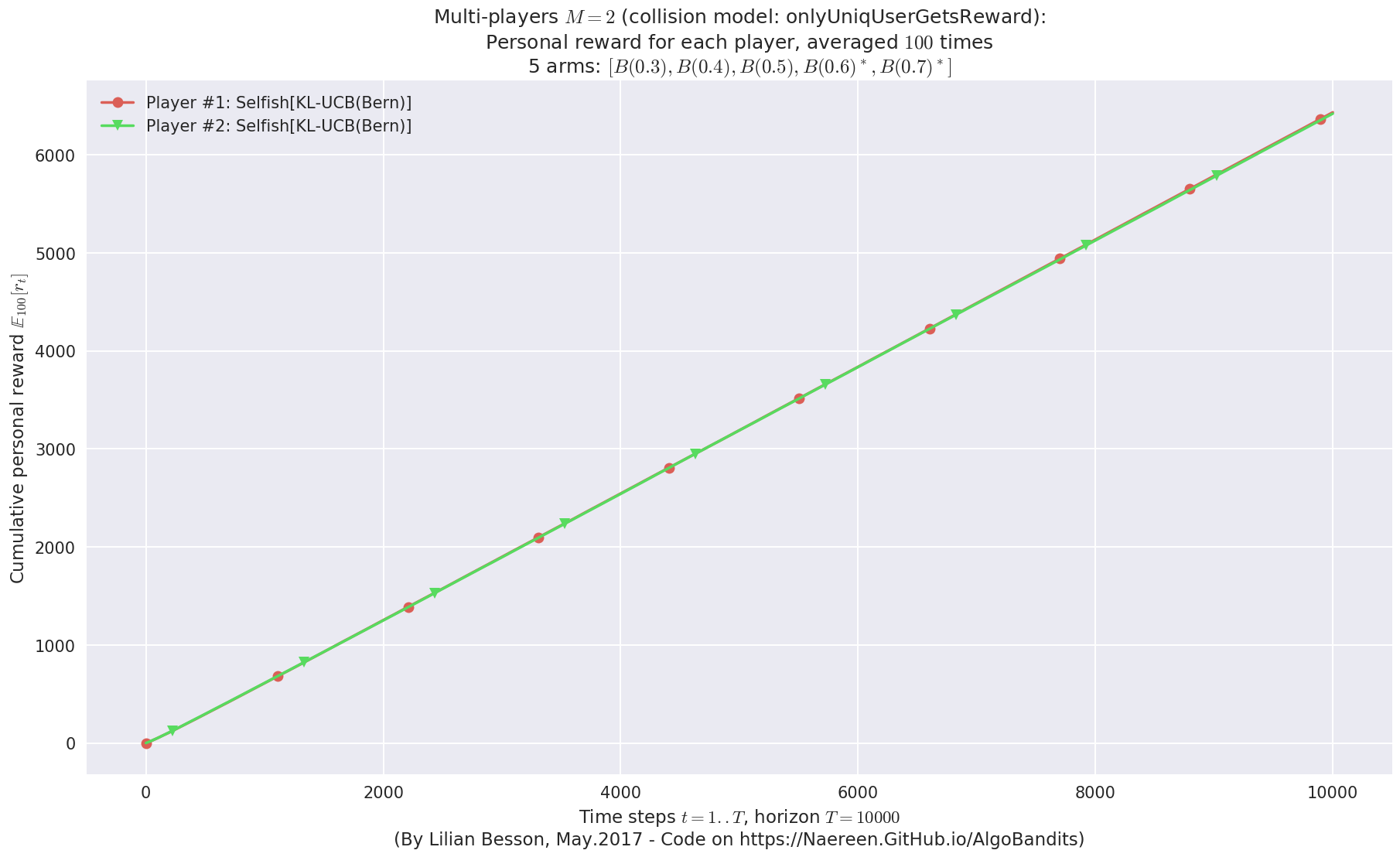
Final ranking for this environment #0 :
- Player #1, '#1<Selfish[KL-UCB(Bern)]>'  was ranked      1 / 2 for this simulation (last rewards = 6402.69).
- Player #2, '#2<Selfish[KL-UCB(Bern)]>'  was ranked      2 / 2 for this simulation (last rewards = 6389.94).
 -  For 2 players, Anandtharam et al. centralized lower-bound gave = 9 ...
 -  For 2 players, our lower bound gave = 18 ...
 -  For 2 players, the initial lower bound in Theorem 6 from [Anandkumar et al., 2010] gave = 12.1 ...

This MAB problem has:
 - a [Lai & Robbins] complexity constant C(mu) = 9.46 for 1-player problem ...
 - a Optimal Arm Identification factor H_OI(mu) = 60.00% ...
 - [Anandtharam et al] centralized lowerbound = 18,
 - Our decentralized lowerbound = 12.1,
 - [Anandkumar et al] decentralized lowerbound = 9
No upper bound for the non-cumulated number of collisions...
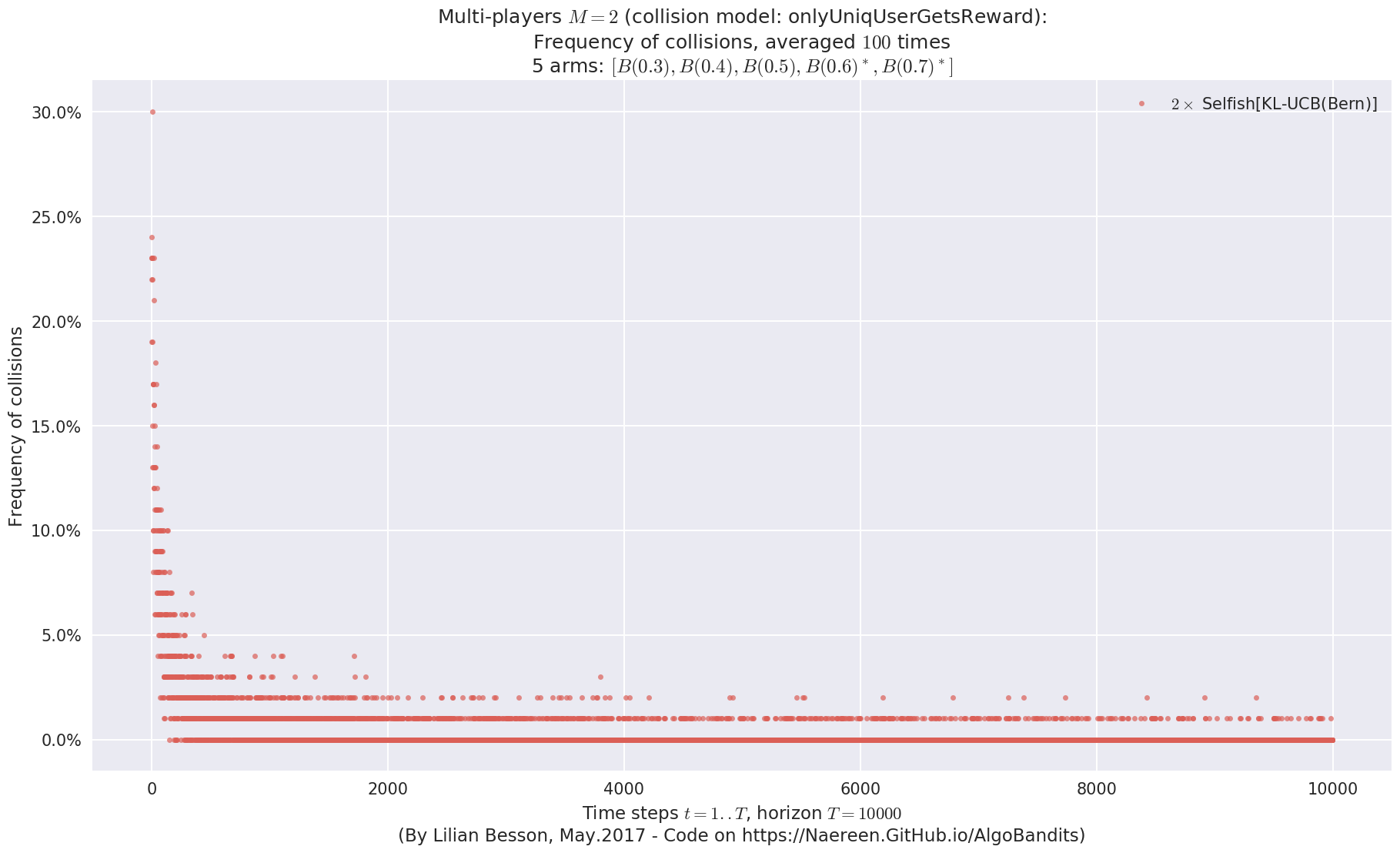
No upper bound for the non-cumulated number of collisions...
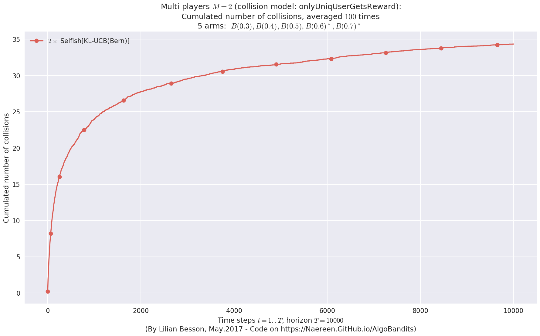
  - For #$0$: $B(0.3)$ ($0.0%$$\%$),    frequency of collisions is 8.7e-05  ...
  - For #$1$: $B(0.4)$ ($0.0%$$\%$),    frequency of collisions is 0.000161  ...
  - For #$2$: $B(0.5)$ ($0.0%$$\%$),    frequency of collisions is 0.000326  ...
  - For #$3$: $B(0.6)$ ($0.1%$$\%$),    frequency of collisions is 0.001005  ...
  - For #$4$: $B(0.7)$ ($0.2%$$\%$),    frequency of collisions is 0.001855  ...

Second problem
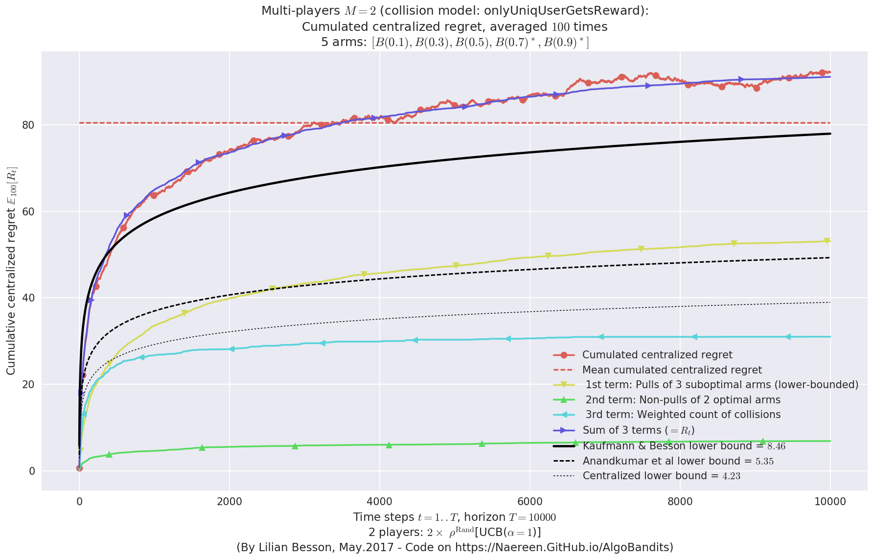
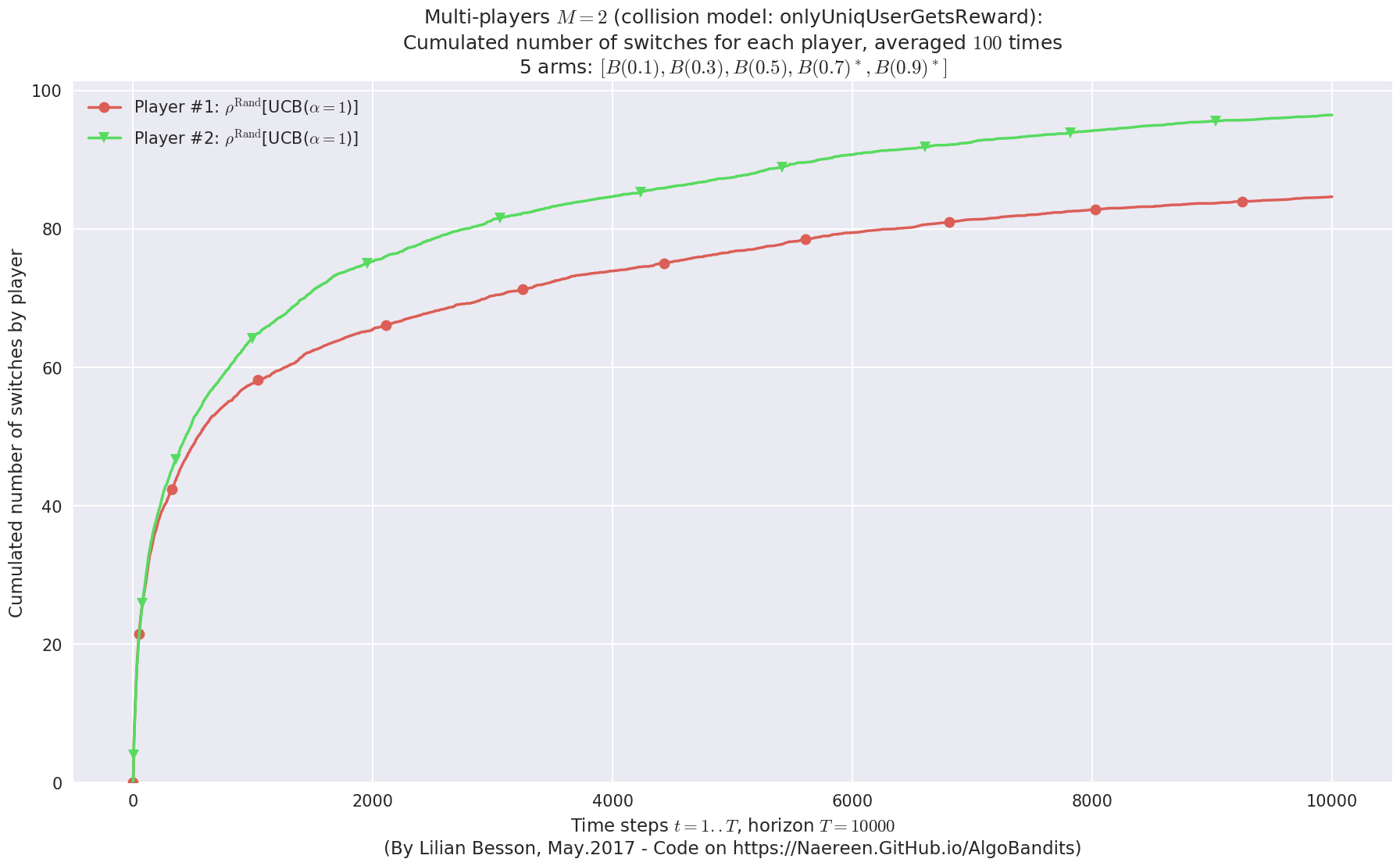
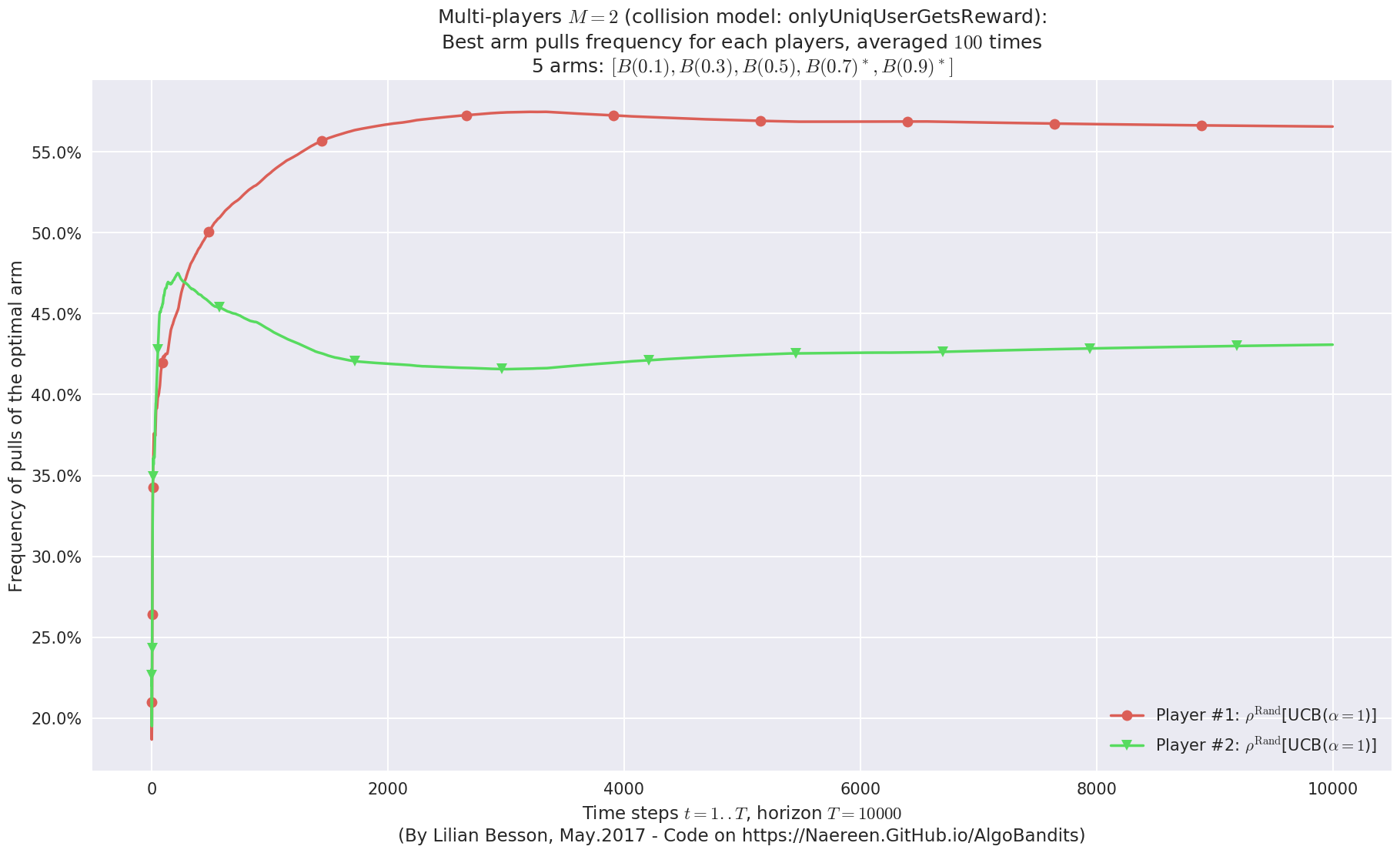
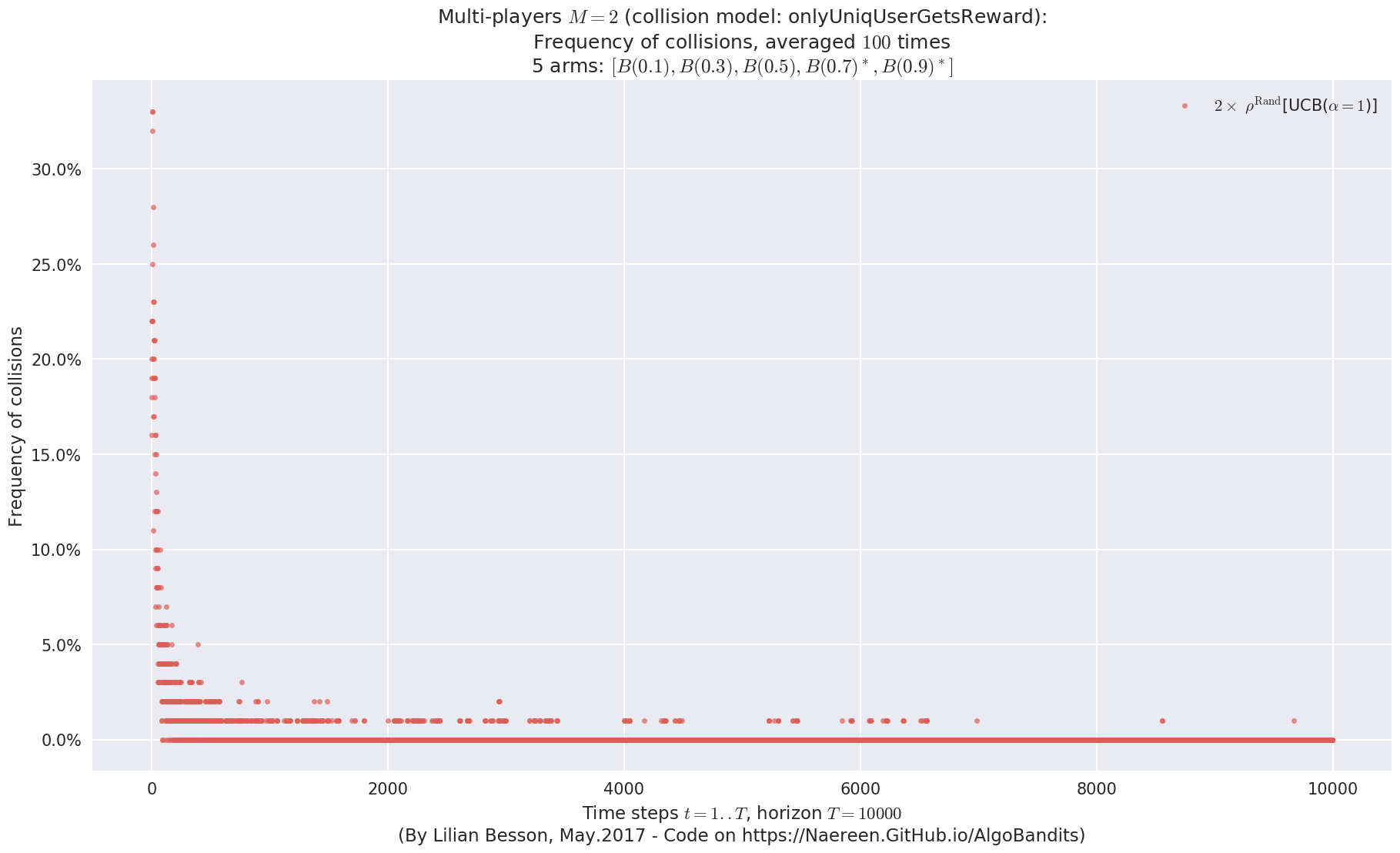
\(\mu = [0.1, 0.3, 0.5, 0.7, 0.9]\) was an easier Bernoulli problem, with larger gap \(\Delta = 0.2\).
In [26]:
for playersId in tqdm(range(len(evs)), desc="Policies"):
    evaluation = evaluators[1][playersId]
    plotAll(evaluation, 1)
Final ranking for this environment #1 :
- Player #1, '#1<$\rho^{\mathrm{Rand}}$[UCB($\alpha=1$)]>'        was ranked      1 / 2 for this simulation (last rewards = 8053.13).
- Player #2, '#2<$\rho^{\mathrm{Rand}}$[UCB($\alpha=1$)]>'        was ranked      2 / 2 for this simulation (last rewards = 7776.4).
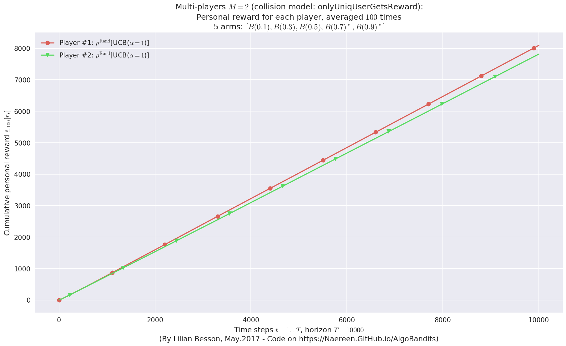
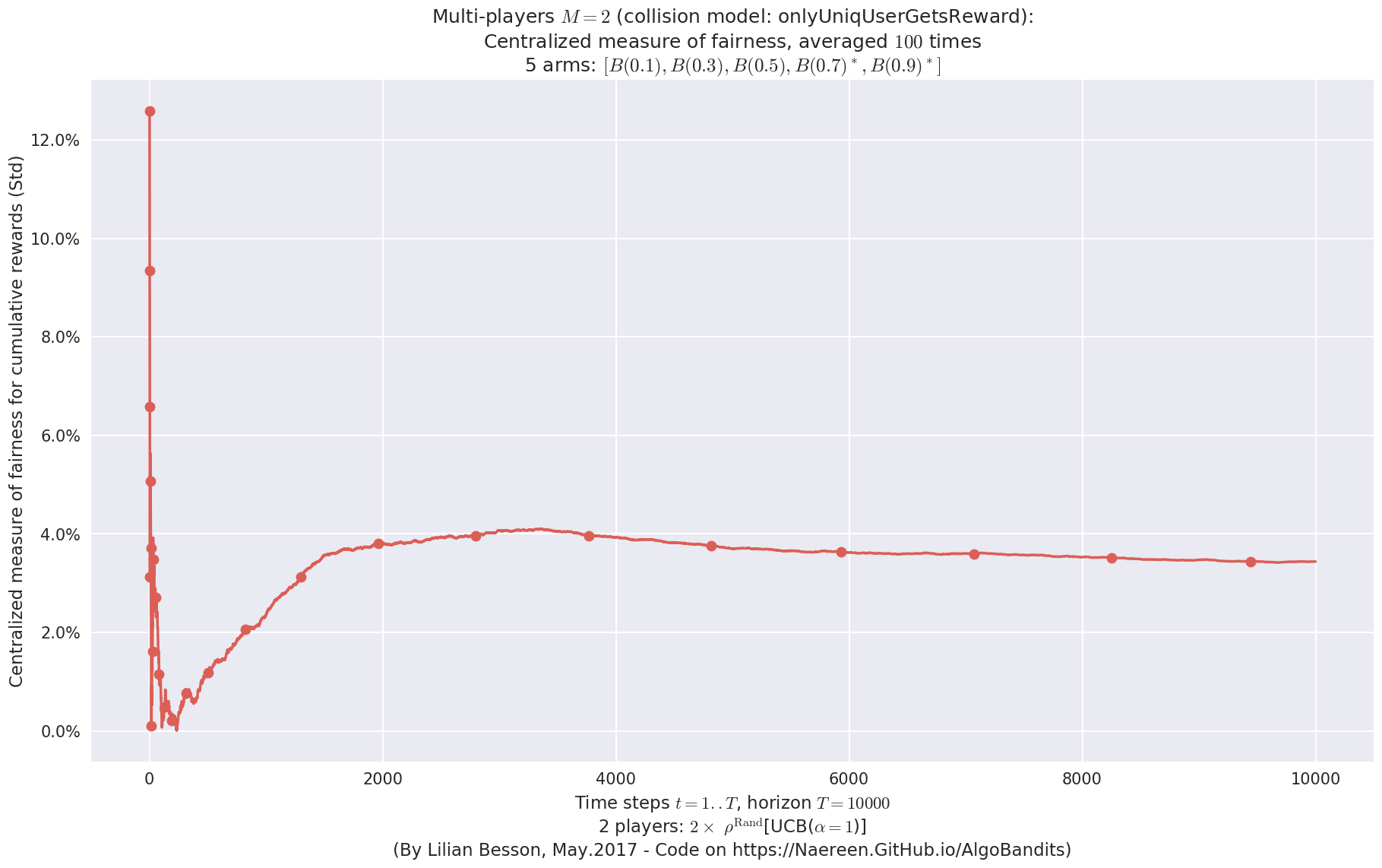
 -  For 2 players, Anandtharam et al. centralized lower-bound gave = 4.23 ...
 -  For 2 players, our lower bound gave = 8.46 ...
 -  For 2 players, the initial lower bound in Theorem 6 from [Anandkumar et al., 2010] gave = 5.35 ...

This MAB problem has:
 - a [Lai & Robbins] complexity constant C(mu) = 3.12 for 1-player problem ...
 - a Optimal Arm Identification factor H_OI(mu) = 40.00% ...
 - [Anandtharam et al] centralized lowerbound = 8.46,
 - Our decentralized lowerbound = 5.35,
 - [Anandkumar et al] decentralized lowerbound = 4.23
No upper bound for the non-cumulated number of collisions...
No upper bound for the non-cumulated number of collisions...
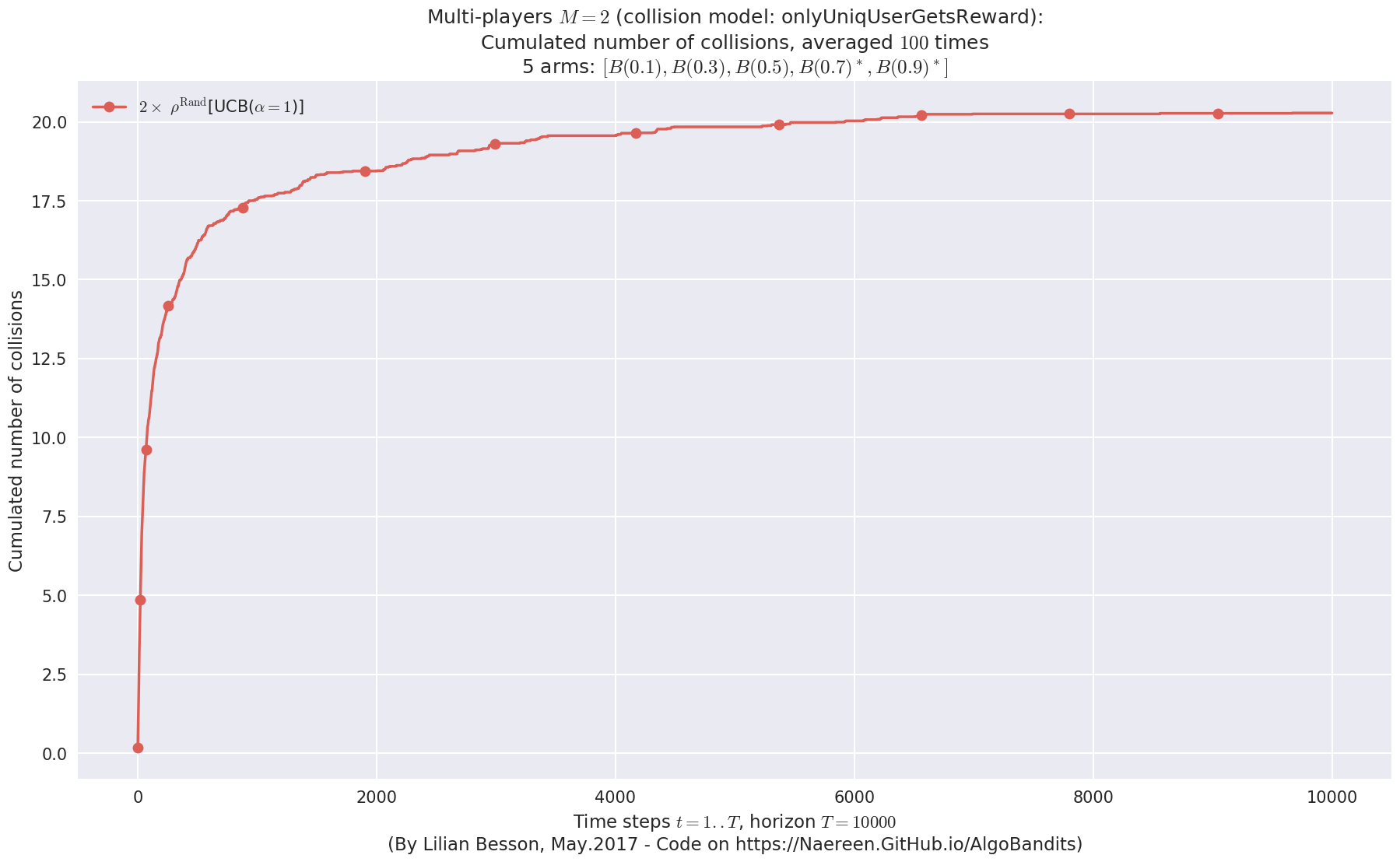
  - For #$0$: $B(0.1)$ ($0.0%$$\%$),    frequency of collisions is 3e-05  ...
  - For #$1$: $B(0.3)$ ($0.0%$$\%$),    frequency of collisions is 5.7e-05  ...
  - For #$2$: $B(0.5)$ ($0.0%$$\%$),    frequency of collisions is 0.000134  ...
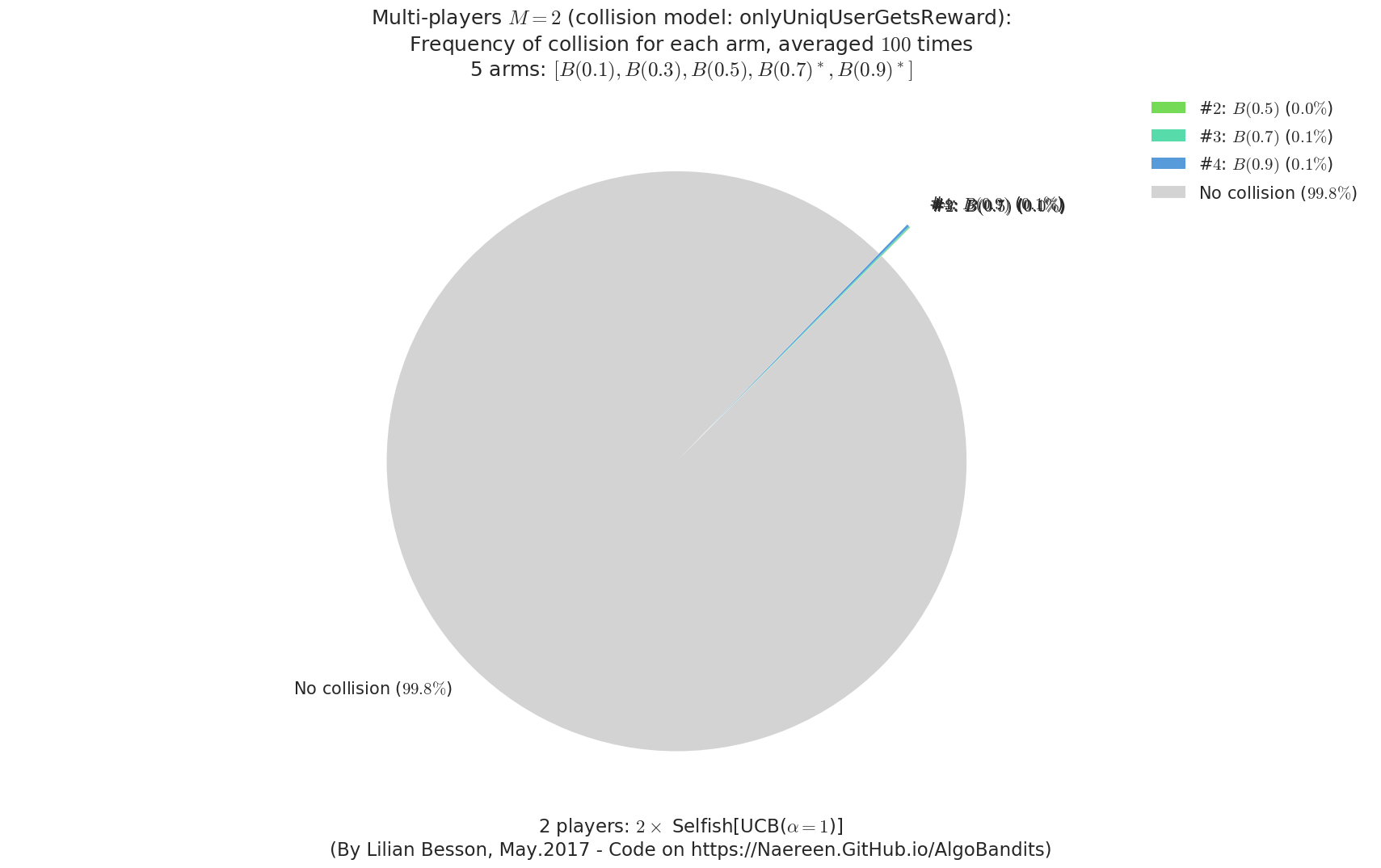
  - For #$3$: $B(0.7)$ ($0.1%$$\%$),    frequency of collisions is 0.000812  ...
  - For #$4$: $B(0.9)$ ($0.1%$$\%$),    frequency of collisions is 0.000995  ...

Final ranking for this environment #1 :
- Player #2, '#2<Selfish[UCB($\alpha=1$)]>'       was ranked      1 / 2 for this simulation (last rewards = 8050.82).
- Player #1, '#1<Selfish[UCB($\alpha=1$)]>'       was ranked      2 / 2 for this simulation (last rewards = 7779.52).
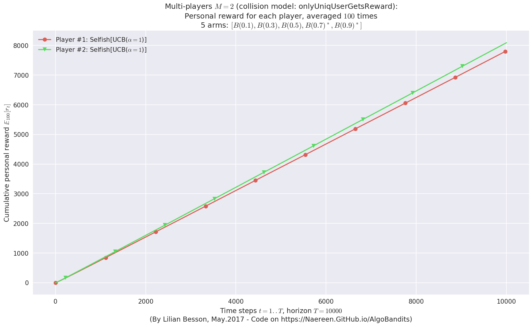
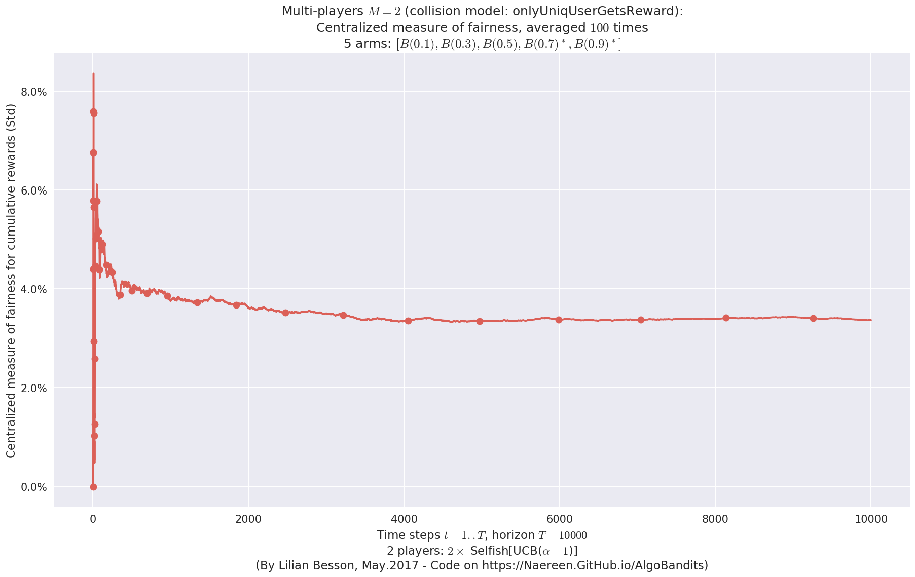
 -  For 2 players, Anandtharam et al. centralized lower-bound gave = 4.23 ...
 -  For 2 players, our lower bound gave = 8.46 ...
 -  For 2 players, the initial lower bound in Theorem 6 from [Anandkumar et al., 2010] gave = 5.35 ...

This MAB problem has:
 - a [Lai & Robbins] complexity constant C(mu) = 3.12 for 1-player problem ...
 - a Optimal Arm Identification factor H_OI(mu) = 40.00% ...
 - [Anandtharam et al] centralized lowerbound = 8.46,
 - Our decentralized lowerbound = 5.35,
 - [Anandkumar et al] decentralized lowerbound = 4.23
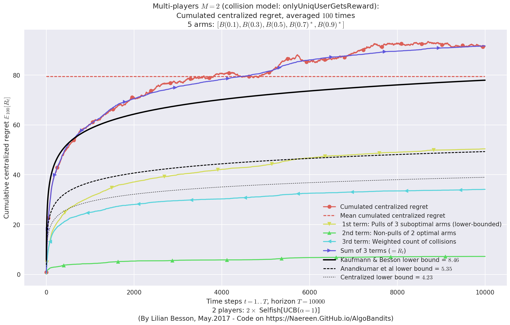
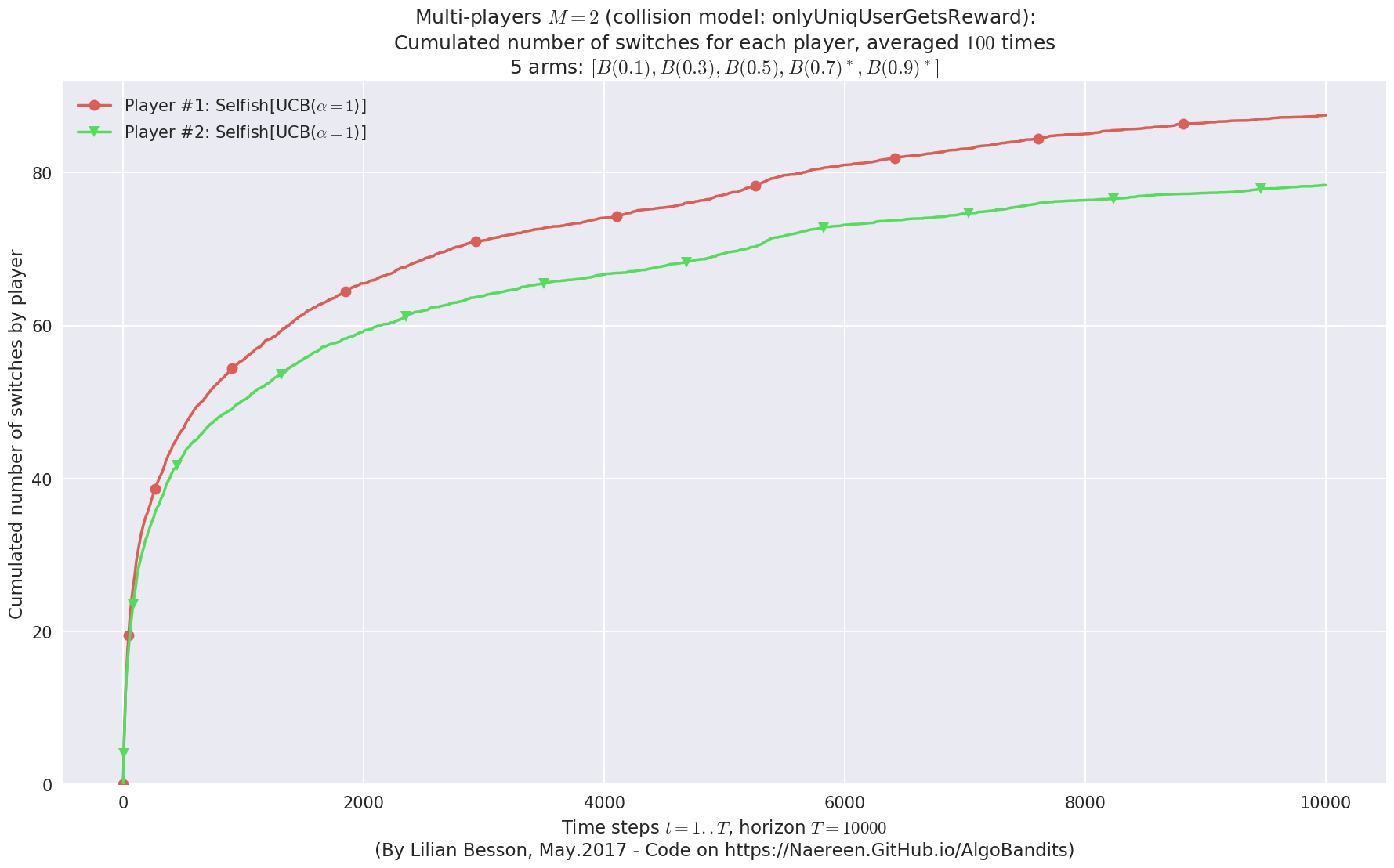
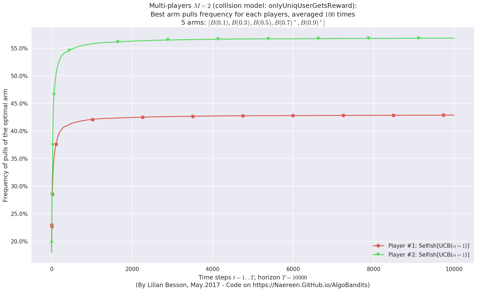
No upper bound for the non-cumulated number of collisions...
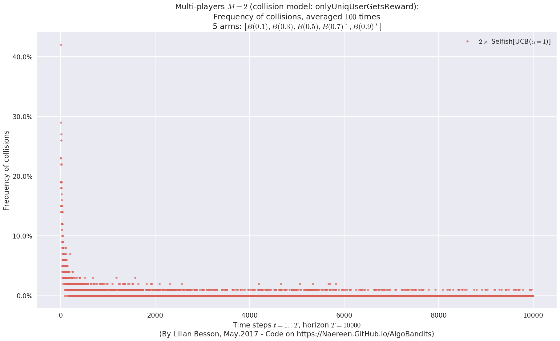
No upper bound for the non-cumulated number of collisions...
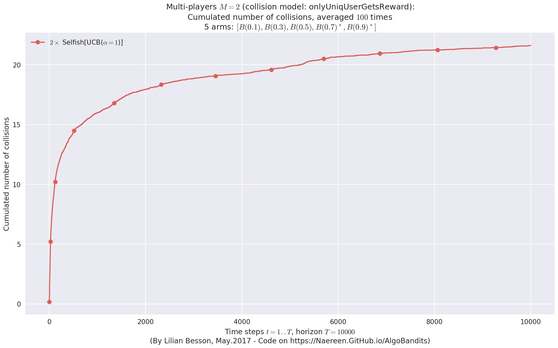
  - For #$0$: $B(0.1)$ ($0.0%$$\%$),    frequency of collisions is 3.5e-05  ...
  - For #$1$: $B(0.3)$ ($0.0%$$\%$),    frequency of collisions is 5.1e-05  ...
  - For #$2$: $B(0.5)$ ($0.0%$$\%$),    frequency of collisions is 0.000143  ...
  - For #$3$: $B(0.7)$ ($0.1%$$\%$),    frequency of collisions is 0.000611  ...
  - For #$4$: $B(0.9)$ ($0.1%$$\%$),    frequency of collisions is 0.00132  ...
Final ranking for this environment #1 :
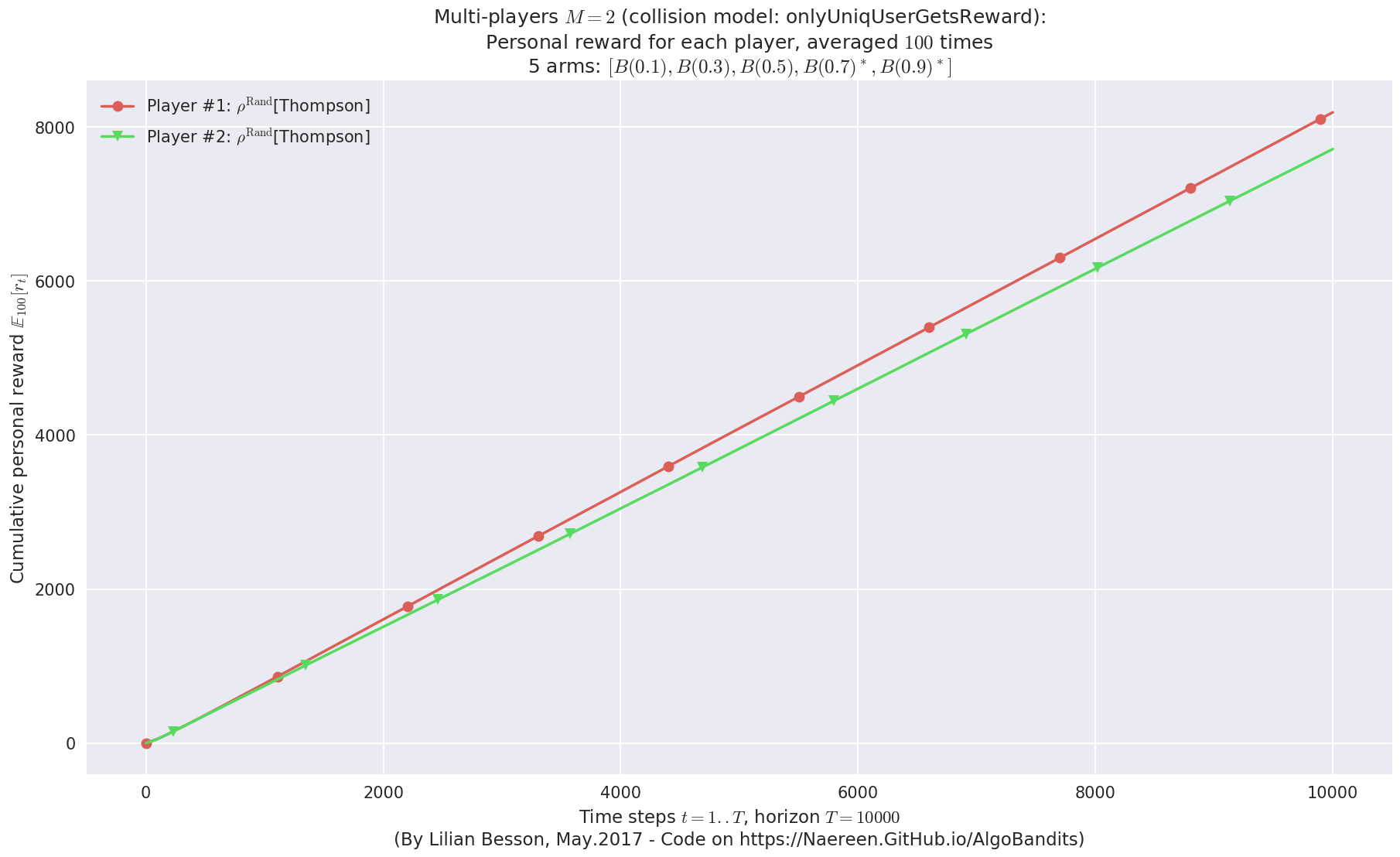
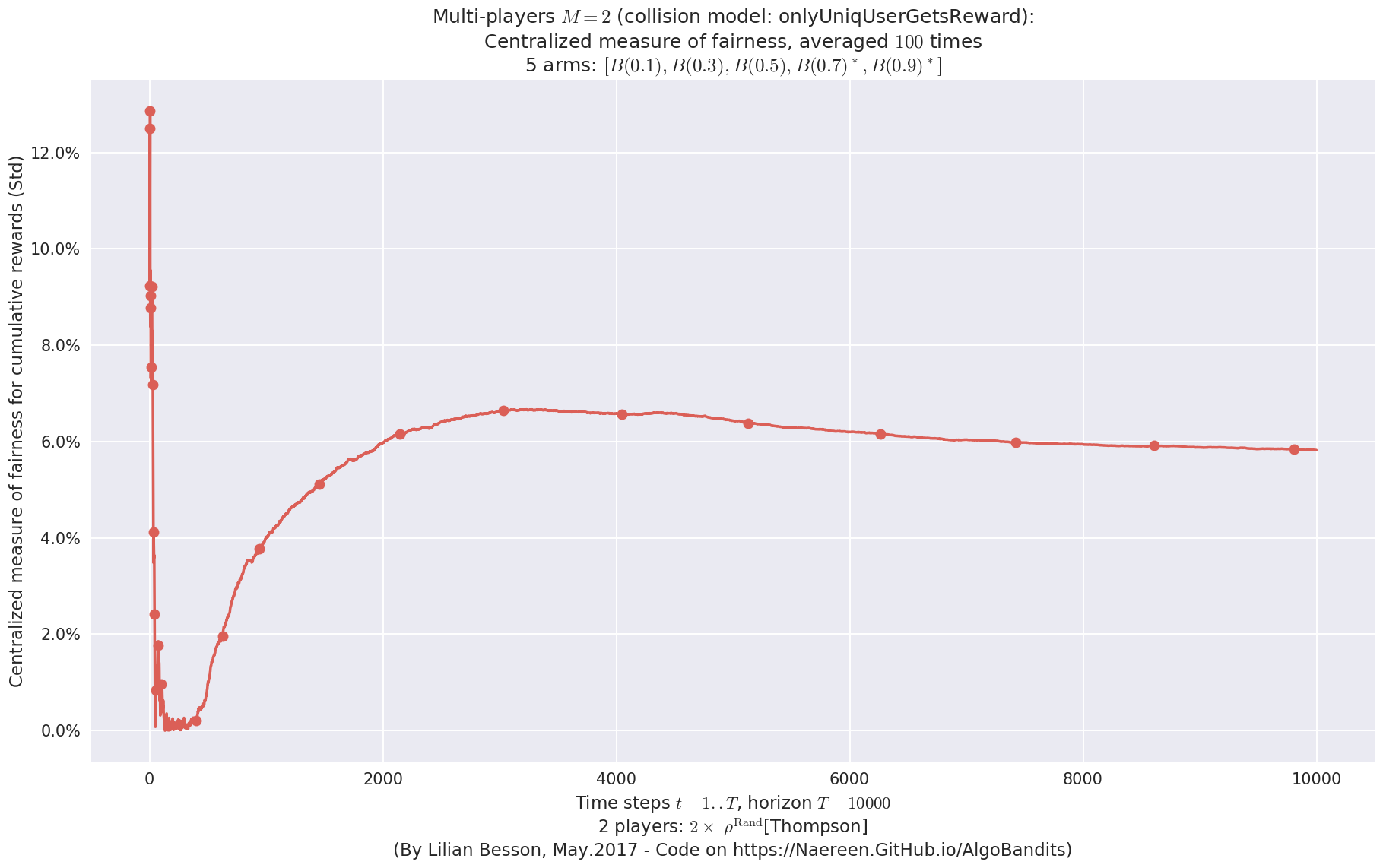
- Player #1, '#1<$\rho^{\mathrm{Rand}}$[Thompson]>'       was ranked      1 / 2 for this simulation (last rewards = 8150.08).
- Player #2, '#2<$\rho^{\mathrm{Rand}}$[Thompson]>'       was ranked      2 / 2 for this simulation (last rewards = 7674.96).
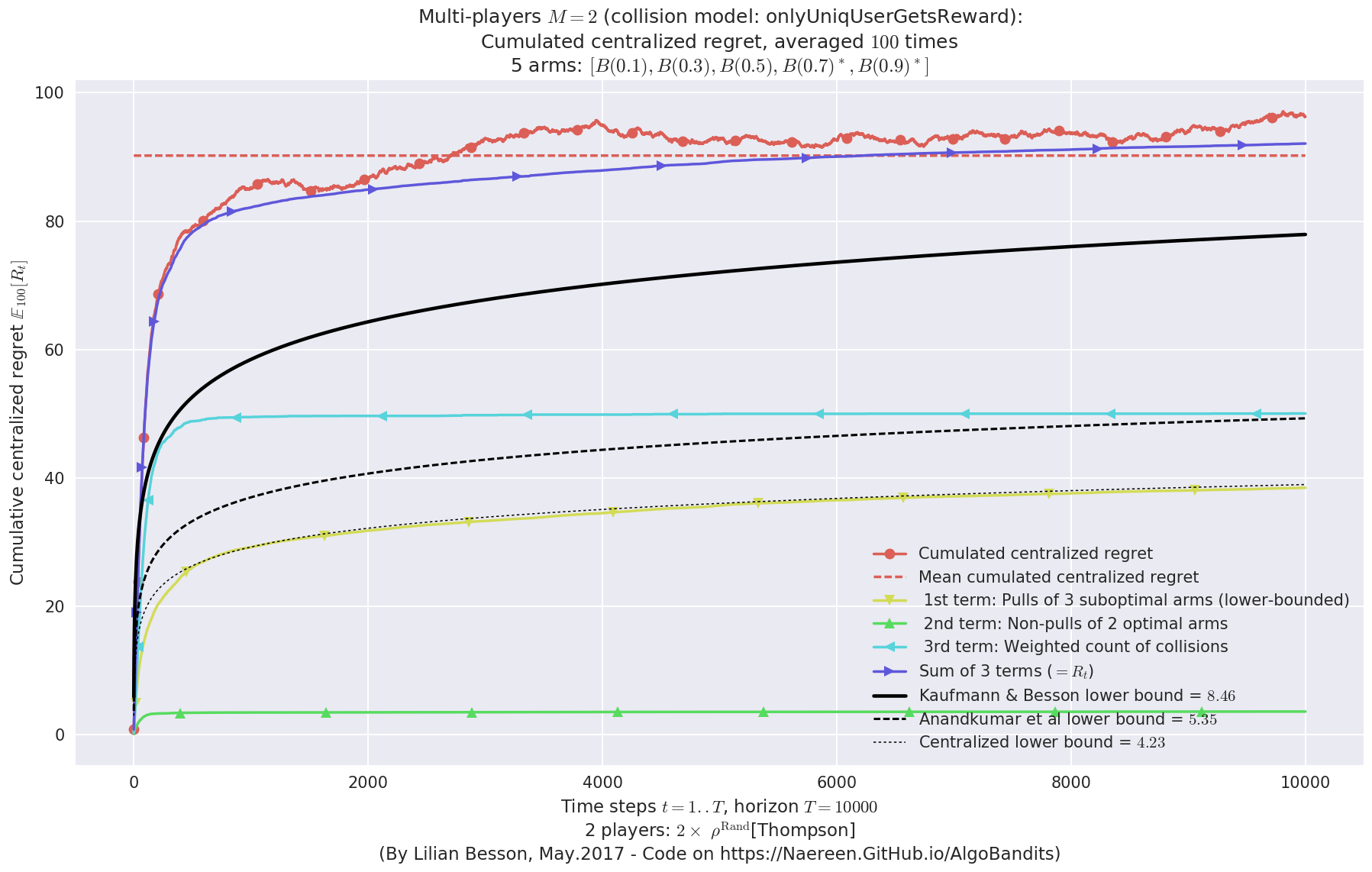
 -  For 2 players, Anandtharam et al. centralized lower-bound gave = 4.23 ...
 -  For 2 players, our lower bound gave = 8.46 ...
 -  For 2 players, the initial lower bound in Theorem 6 from [Anandkumar et al., 2010] gave = 5.35 ...

This MAB problem has:
 - a [Lai & Robbins] complexity constant C(mu) = 3.12 for 1-player problem ...
 - a Optimal Arm Identification factor H_OI(mu) = 40.00% ...
 - [Anandtharam et al] centralized lowerbound = 8.46,
 - Our decentralized lowerbound = 5.35,
 - [Anandkumar et al] decentralized lowerbound = 4.23
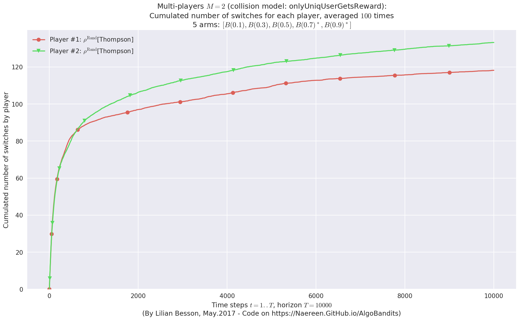
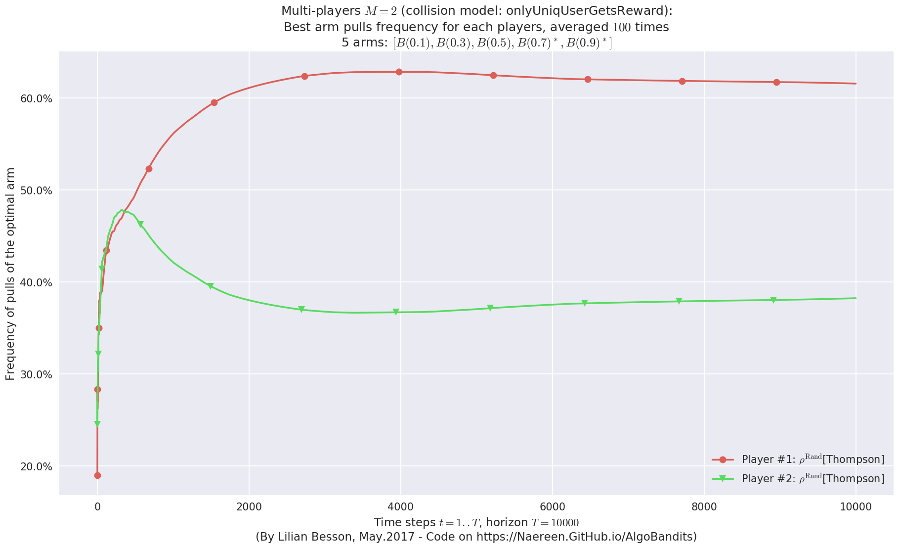
No upper bound for the non-cumulated number of collisions...
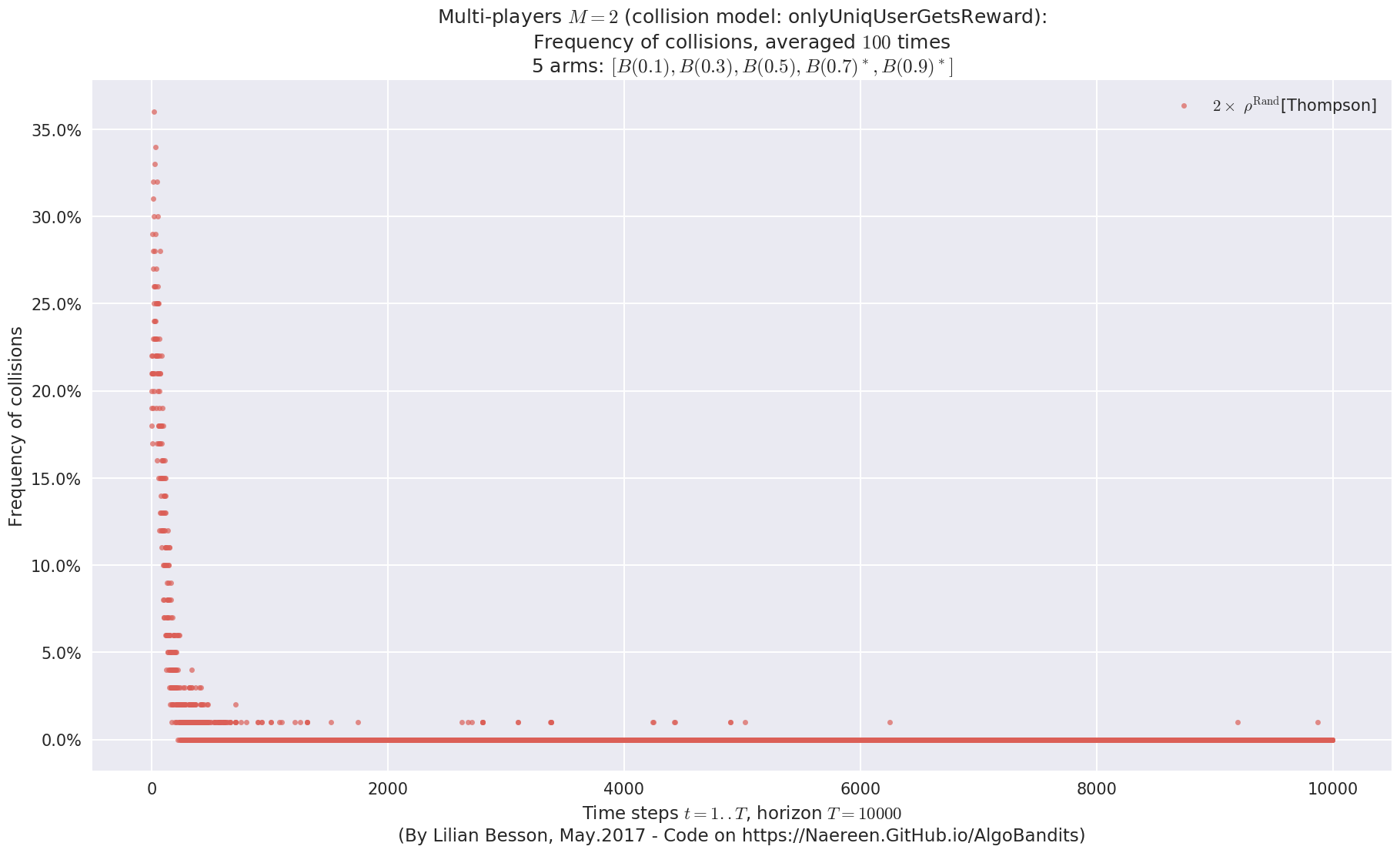
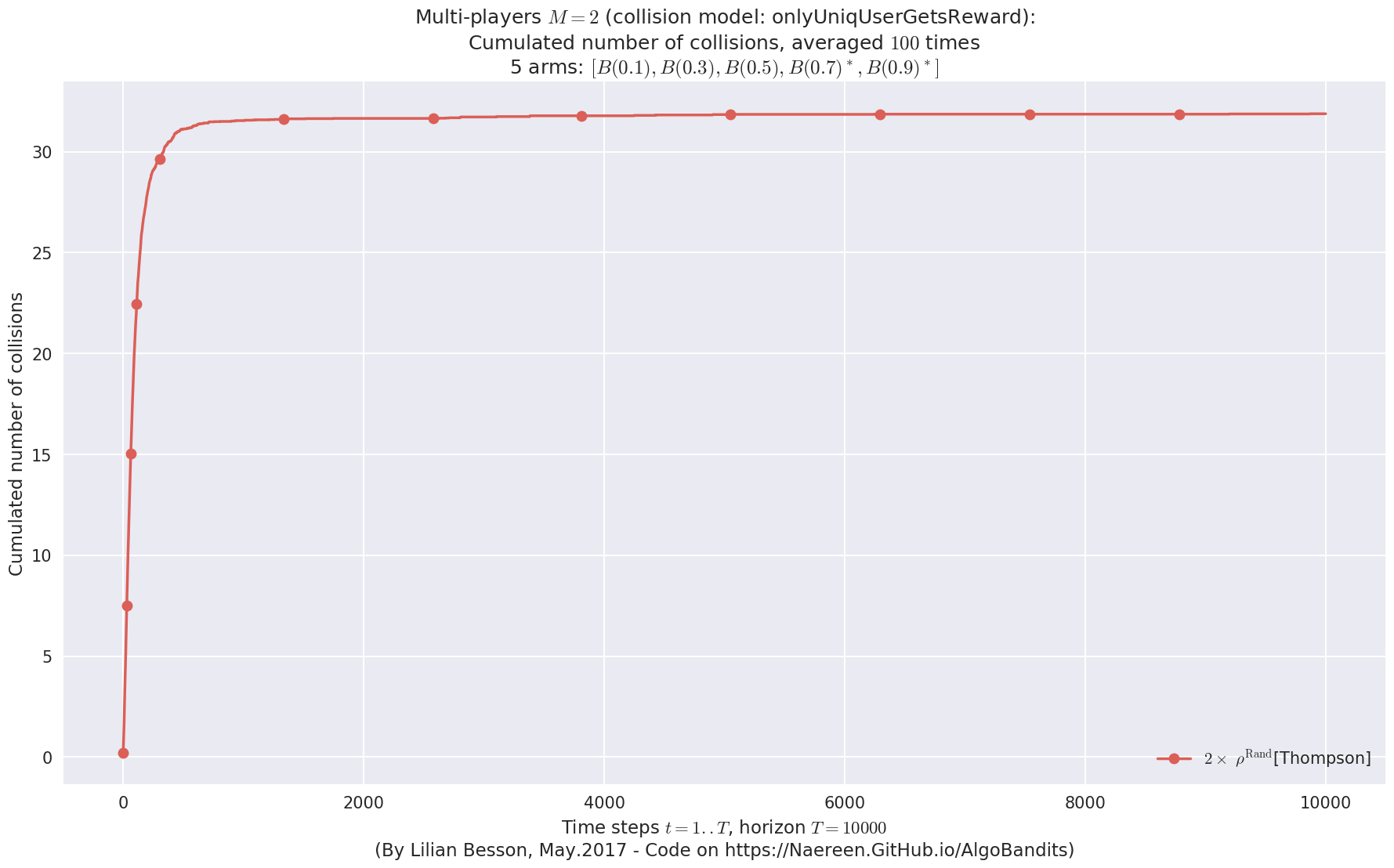
No upper bound for the non-cumulated number of collisions...
  - For #$0$: $B(0.1)$ ($0.0%$$\%$),    frequency of collisions is 2.2e-05  ...
  - For #$1$: $B(0.3)$ ($0.0%$$\%$),    frequency of collisions is 4.7e-05  ...
  - For #$2$: $B(0.5)$ ($0.0%$$\%$),    frequency of collisions is 0.000186  ...
  - For #$3$: $B(0.7)$ ($0.1%$$\%$),    frequency of collisions is 0.001237  ...
  - For #$4$: $B(0.9)$ ($0.2%$$\%$),    frequency of collisions is 0.001696  ...
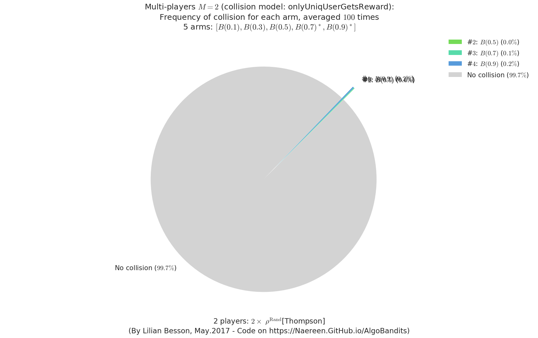
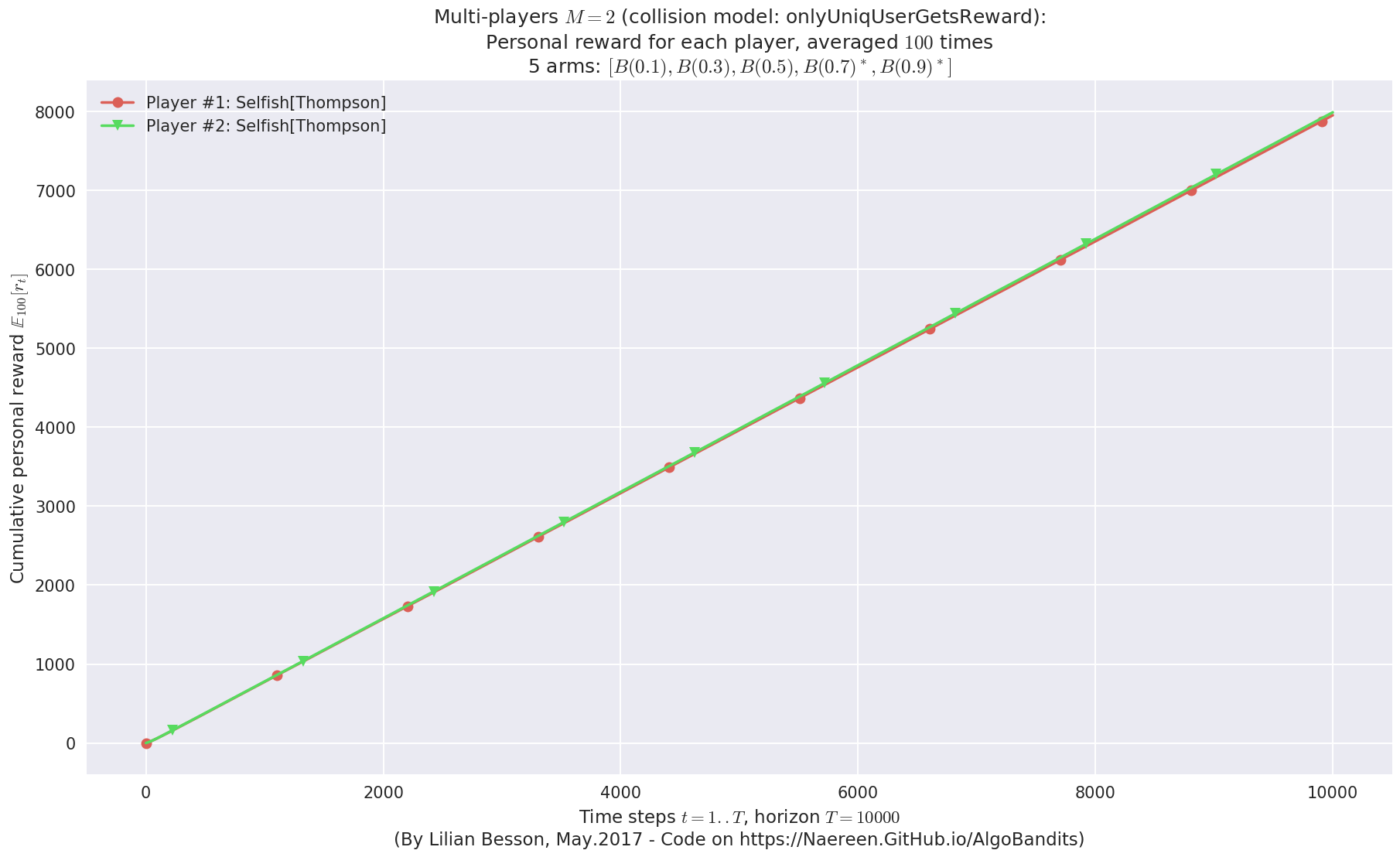
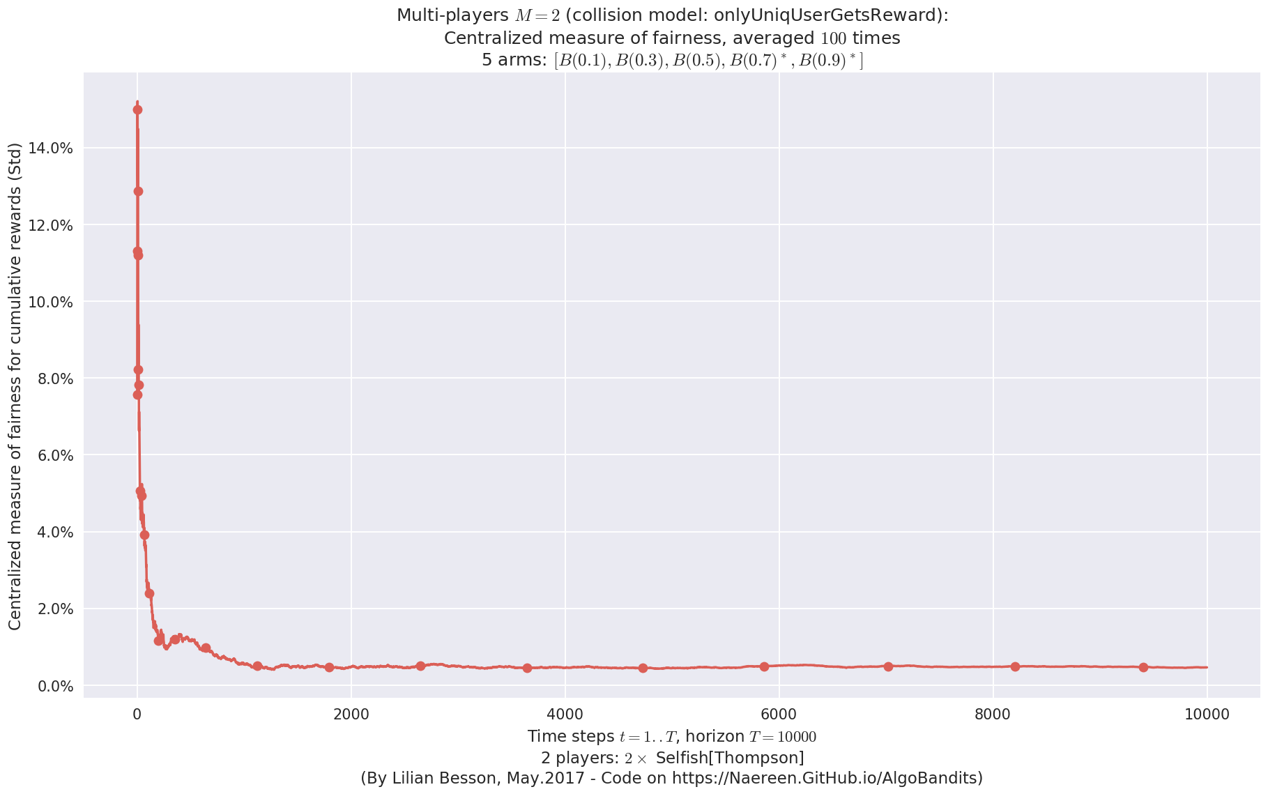
Final ranking for this environment #1 :
- Player #2, '#2<Selfish[Thompson]>'      was ranked      1 / 2 for this simulation (last rewards = 7947.53).
- Player #1, '#1<Selfish[Thompson]>'      was ranked      2 / 2 for this simulation (last rewards = 7910.79).
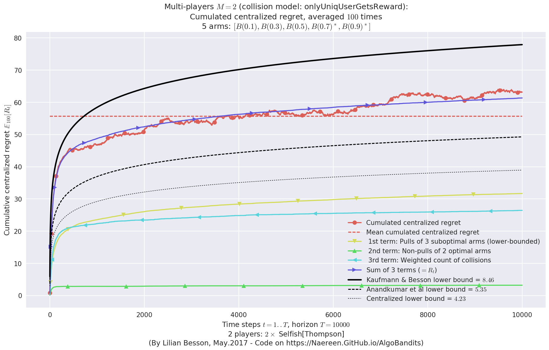
 -  For 2 players, Anandtharam et al. centralized lower-bound gave = 4.23 ...
 -  For 2 players, our lower bound gave = 8.46 ...
 -  For 2 players, the initial lower bound in Theorem 6 from [Anandkumar et al., 2010] gave = 5.35 ...

This MAB problem has:
 - a [Lai & Robbins] complexity constant C(mu) = 3.12 for 1-player problem ...
 - a Optimal Arm Identification factor H_OI(mu) = 40.00% ...
 - [Anandtharam et al] centralized lowerbound = 8.46,
 - Our decentralized lowerbound = 5.35,
 - [Anandkumar et al] decentralized lowerbound = 4.23
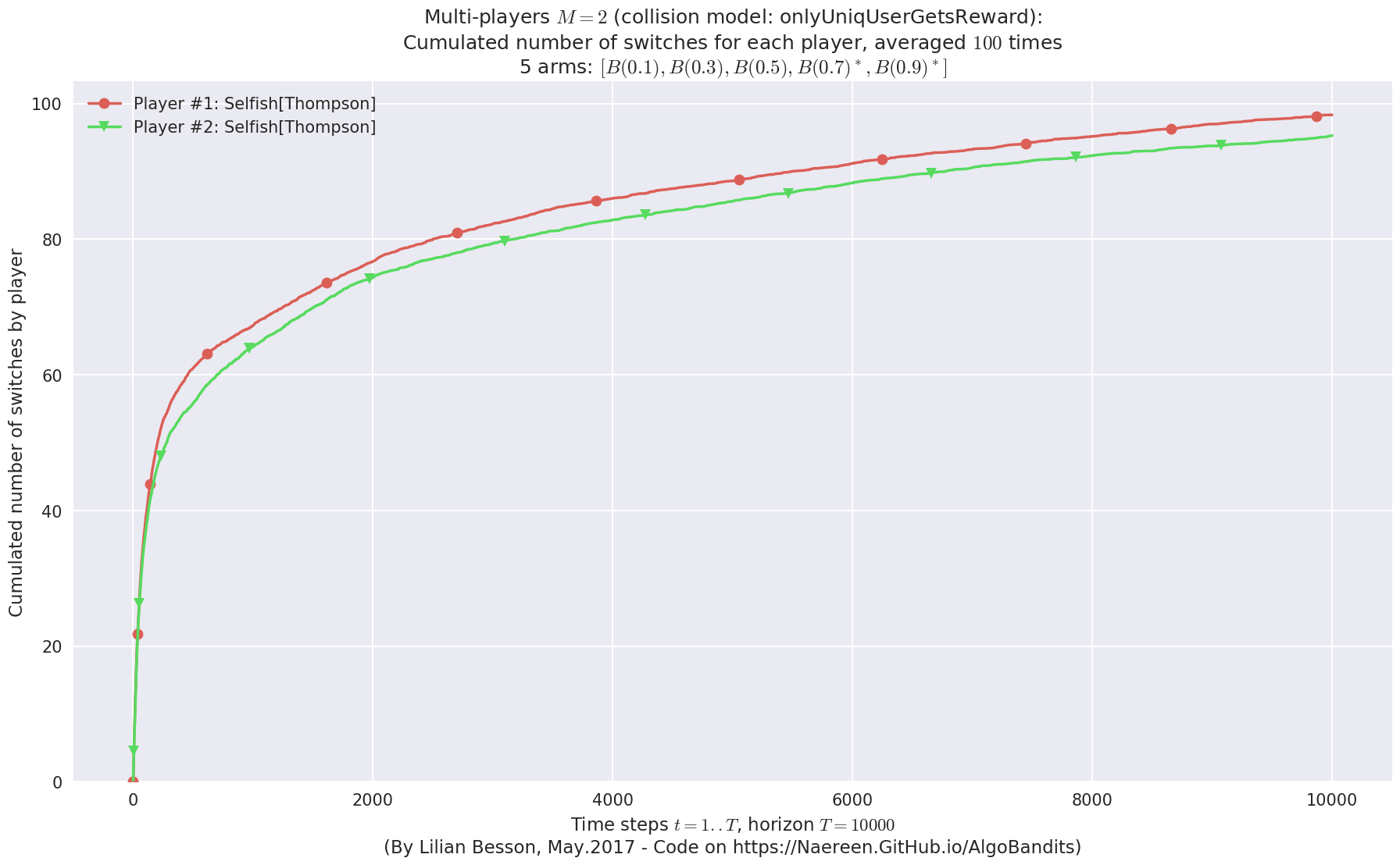
No upper bound for the non-cumulated number of collisions...
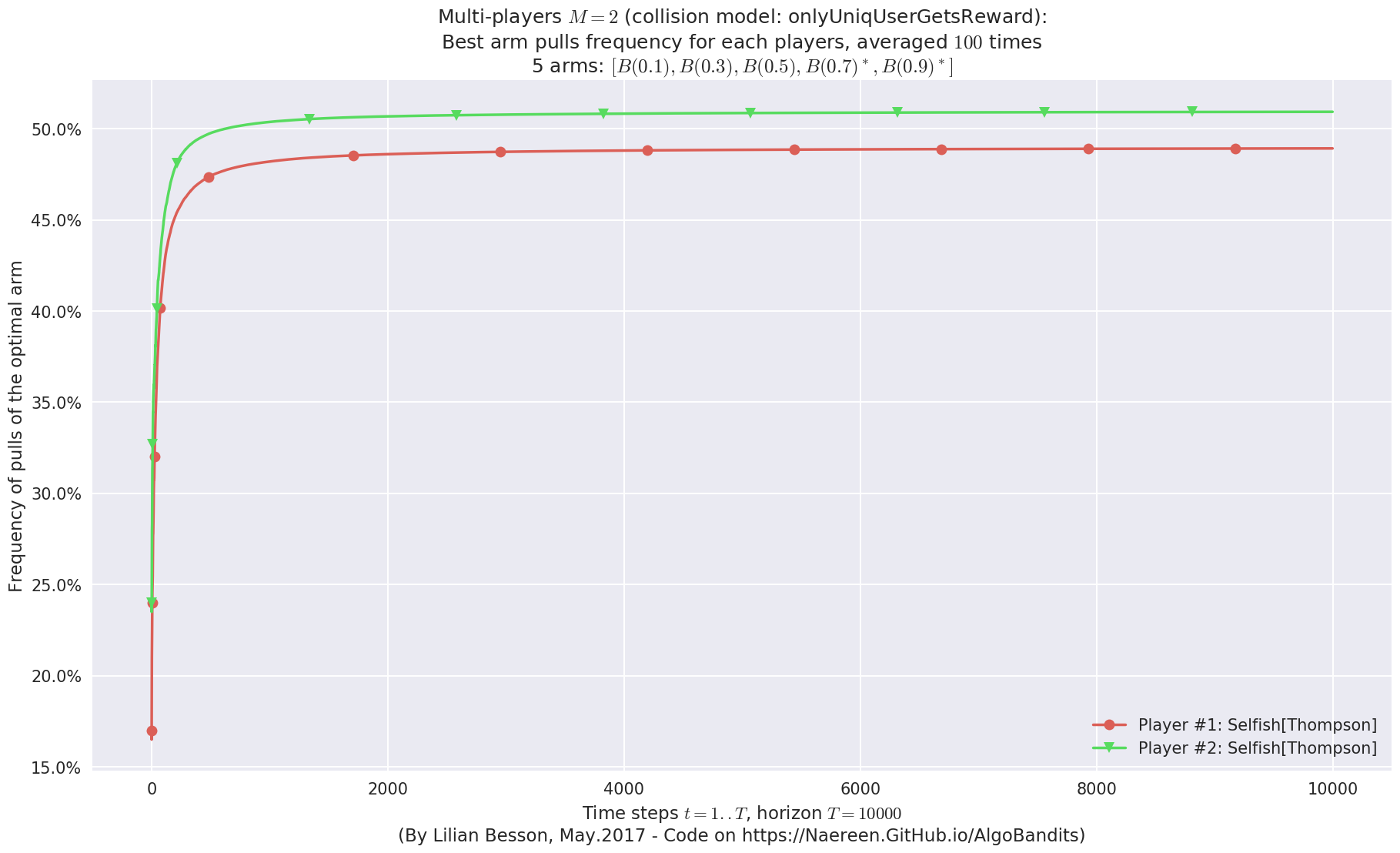
No upper bound for the non-cumulated number of collisions...
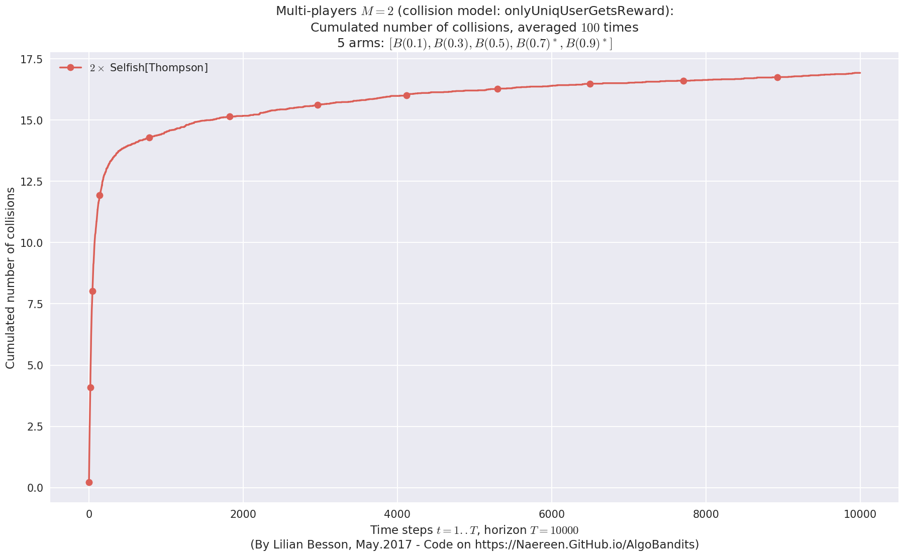
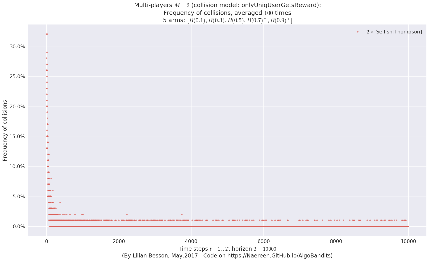
  - For #$0$: $B(0.1)$ ($0.0%$$\%$),    frequency of collisions is 4.2e-05  ...
  - For #$1$: $B(0.3)$ ($0.0%$$\%$),    frequency of collisions is 5.3e-05  ...
  - For #$2$: $B(0.5)$ ($0.0%$$\%$),    frequency of collisions is 0.000139  ...
  - For #$3$: $B(0.7)$ ($0.0%$$\%$),    frequency of collisions is 0.000397  ...
  - For #$4$: $B(0.9)$ ($0.1%$$\%$),    frequency of collisions is 0.001061  ...
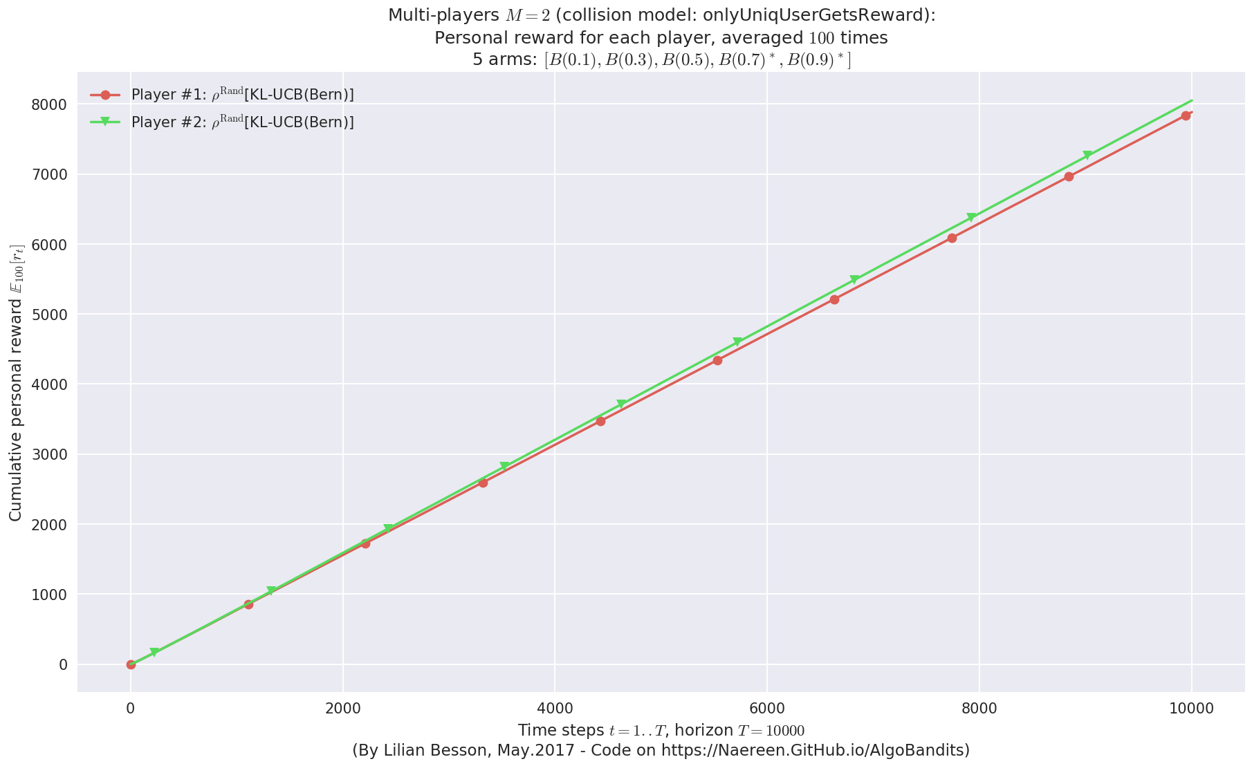
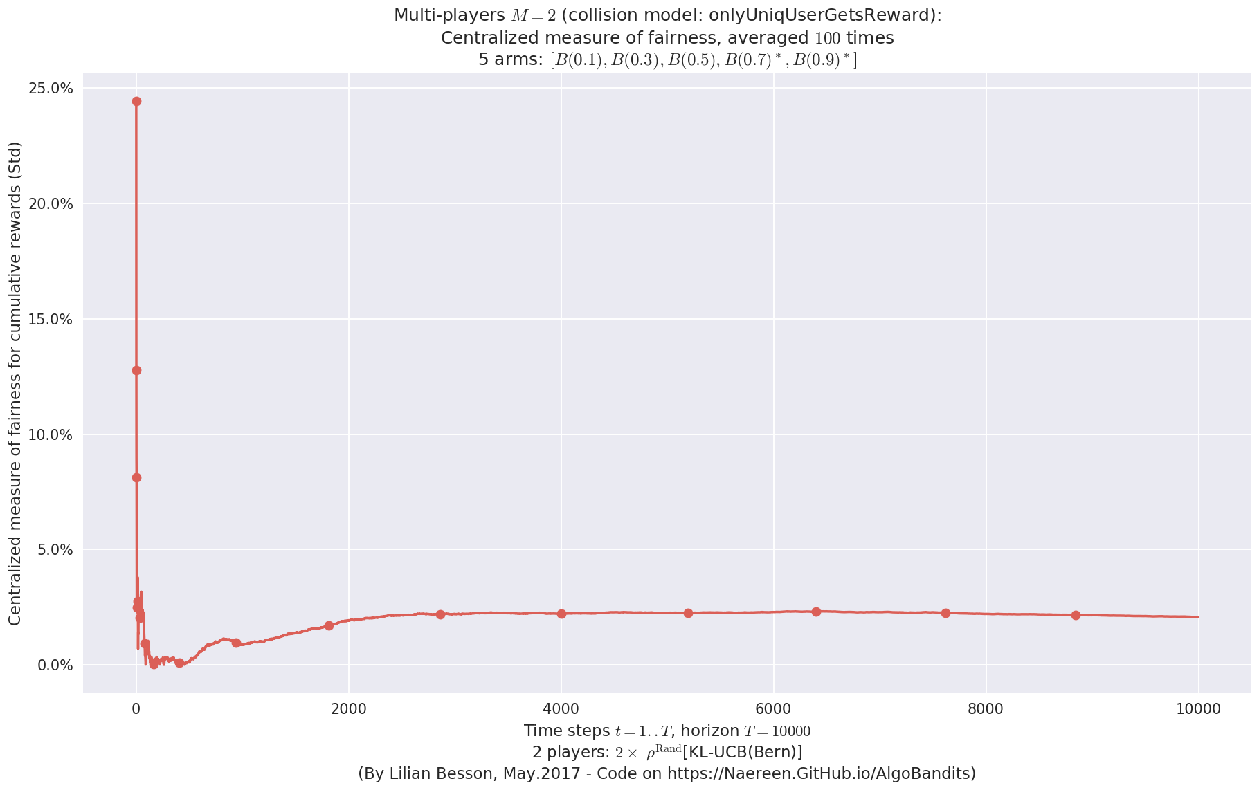
Final ranking for this environment #1 :
- Player #2, '#2<$\rho^{\mathrm{Rand}}$[KL-UCB(Bern)]>'   was ranked      1 / 2 for this simulation (last rewards = 8010.4).
- Player #1, '#1<$\rho^{\mathrm{Rand}}$[KL-UCB(Bern)]>'   was ranked      2 / 2 for this simulation (last rewards = 7844.21).
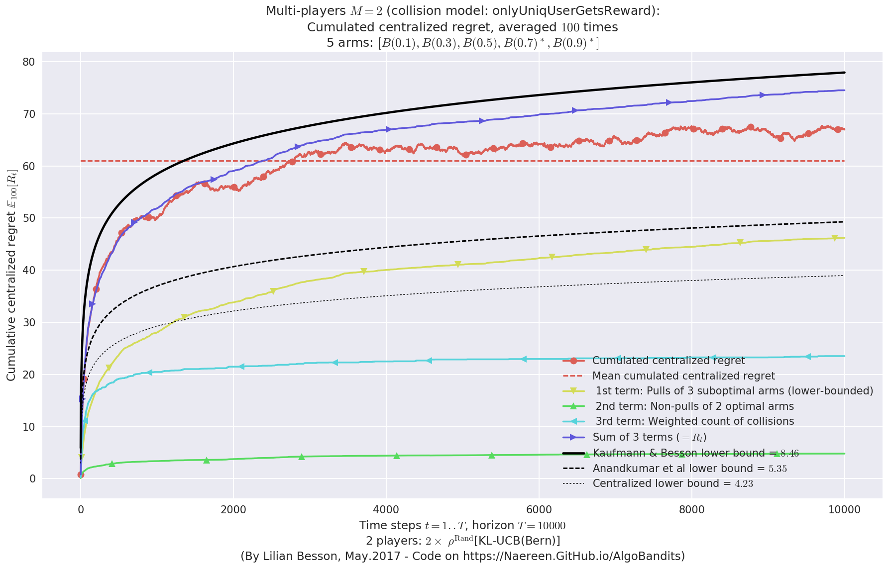
 -  For 2 players, Anandtharam et al. centralized lower-bound gave = 4.23 ...
 -  For 2 players, our lower bound gave = 8.46 ...
 -  For 2 players, the initial lower bound in Theorem 6 from [Anandkumar et al., 2010] gave = 5.35 ...

This MAB problem has:
 - a [Lai & Robbins] complexity constant C(mu) = 3.12 for 1-player problem ...
 - a Optimal Arm Identification factor H_OI(mu) = 40.00% ...
 - [Anandtharam et al] centralized lowerbound = 8.46,
 - Our decentralized lowerbound = 5.35,
 - [Anandkumar et al] decentralized lowerbound = 4.23
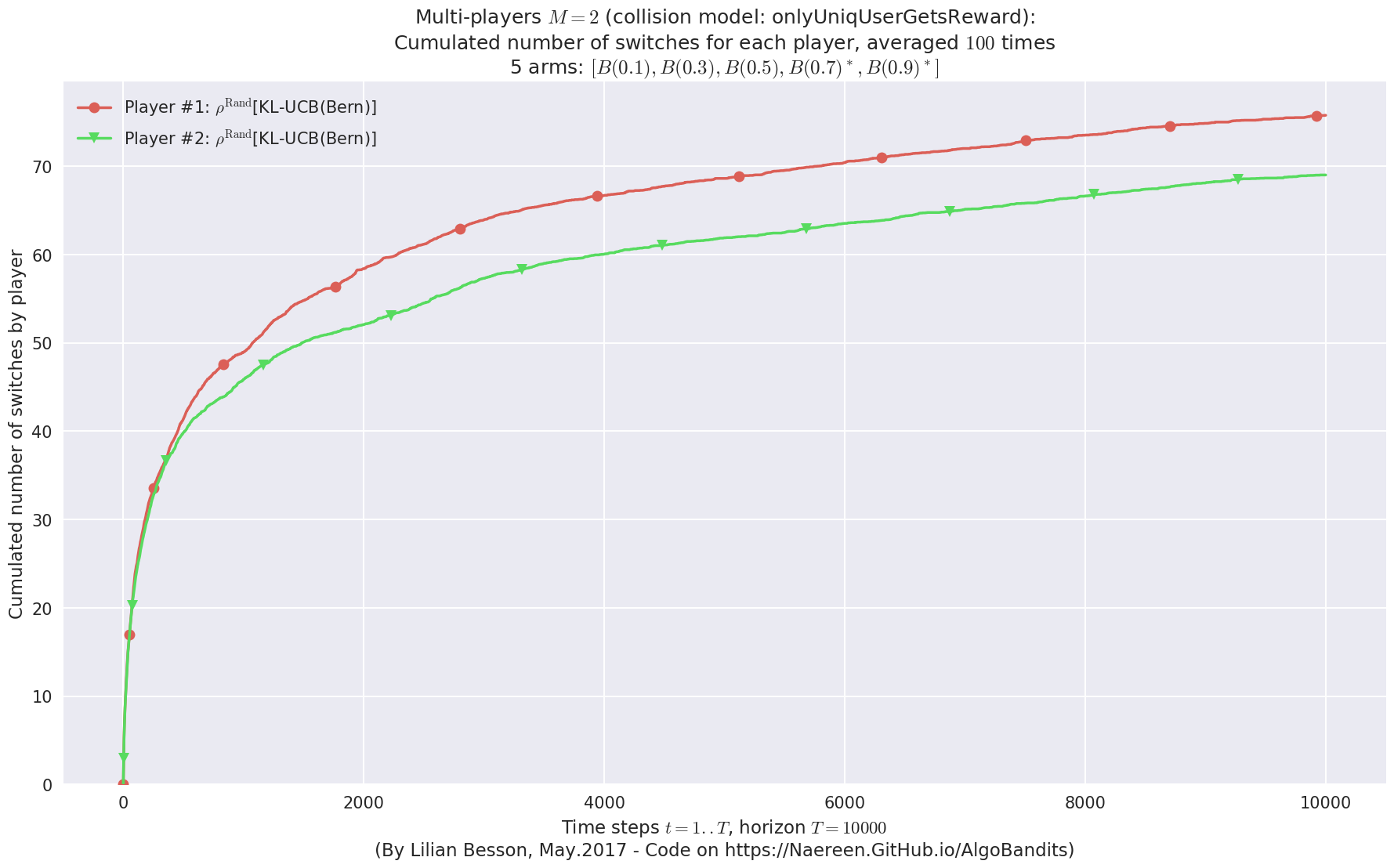
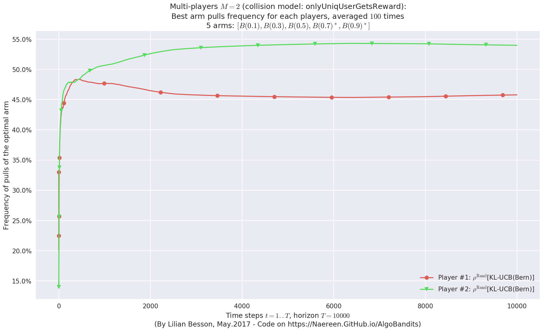
No upper bound for the non-cumulated number of collisions...
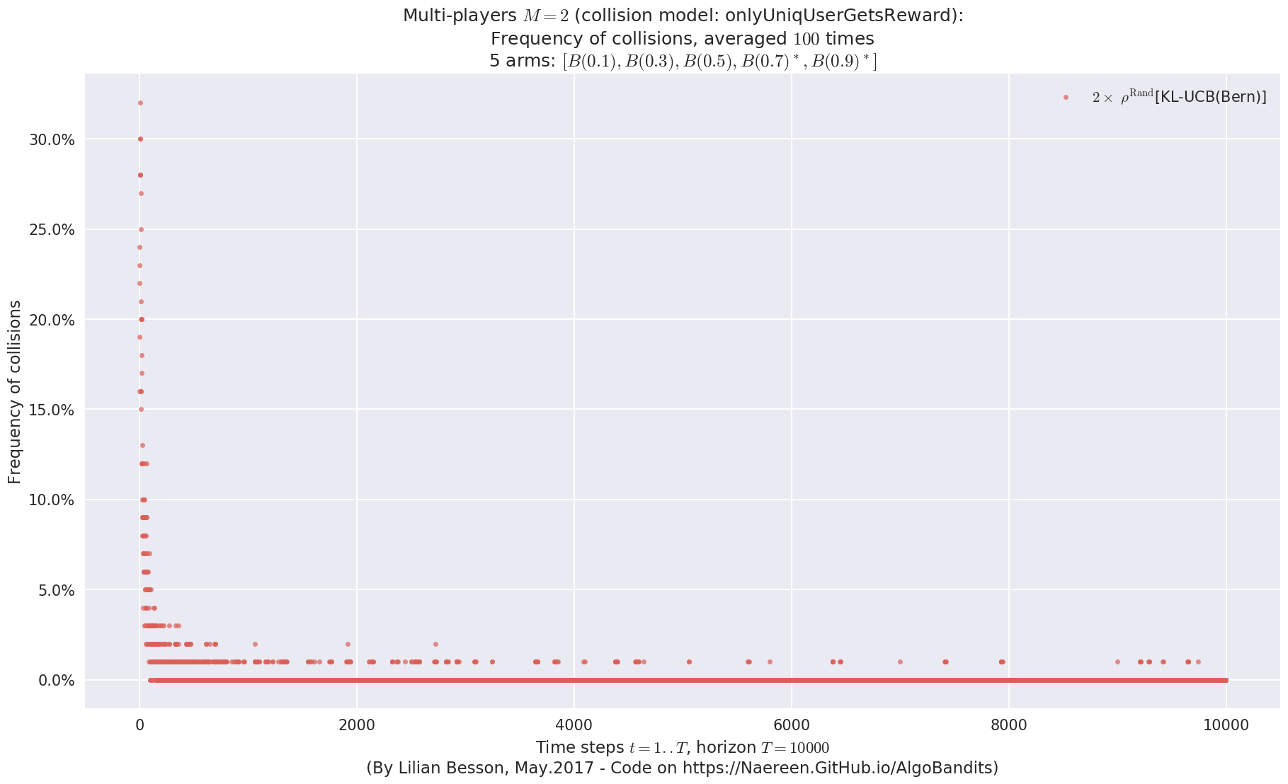
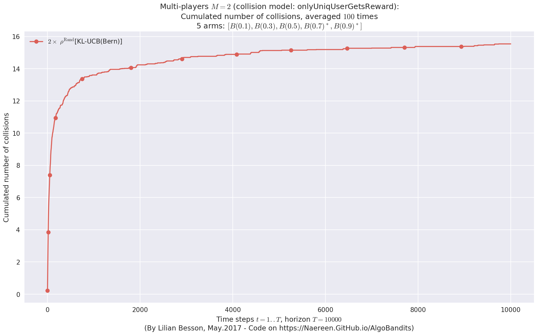
No upper bound for the non-cumulated number of collisions...
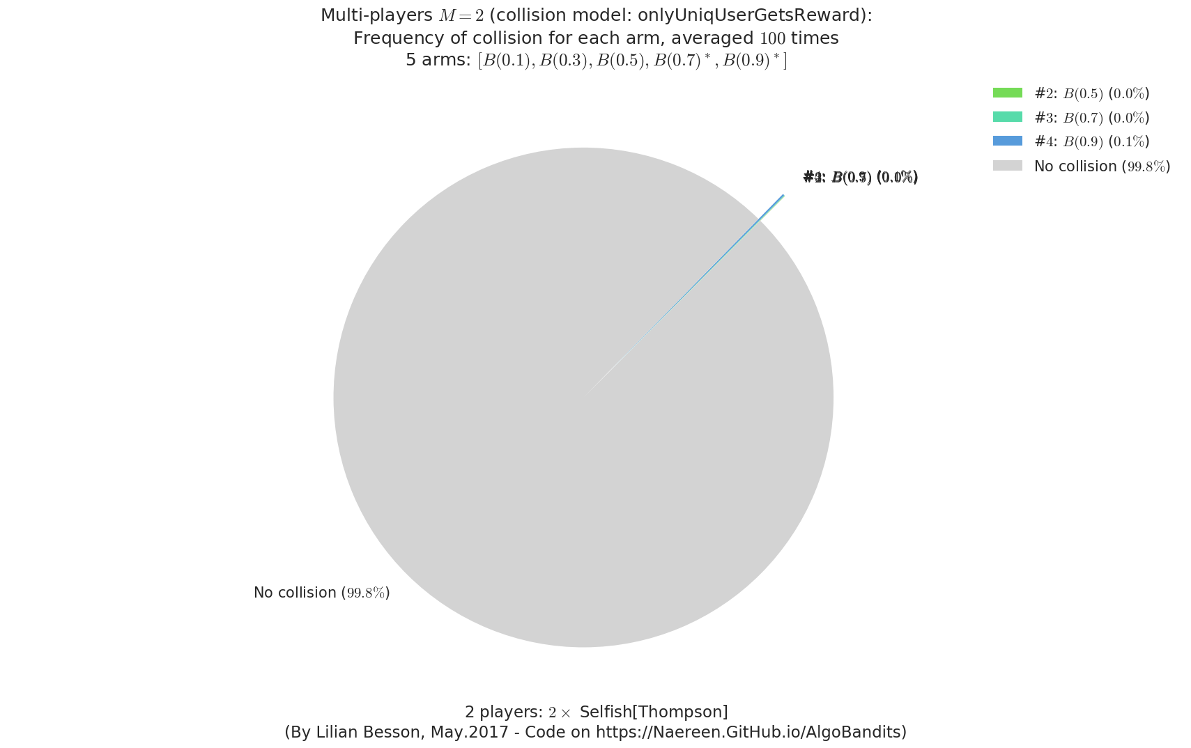
  - For #$0$: $B(0.1)$ ($0.0%$$\%$),    frequency of collisions is 2.5e-05  ...
  - For #$1$: $B(0.3)$ ($0.0%$$\%$),    frequency of collisions is 4.5e-05  ...
  - For #$2$: $B(0.5)$ ($0.0%$$\%$),    frequency of collisions is 0.000144  ...
  - For #$3$: $B(0.7)$ ($0.1%$$\%$),    frequency of collisions is 0.000592  ...
  - For #$4$: $B(0.9)$ ($0.1%$$\%$),    frequency of collisions is 0.000748  ...
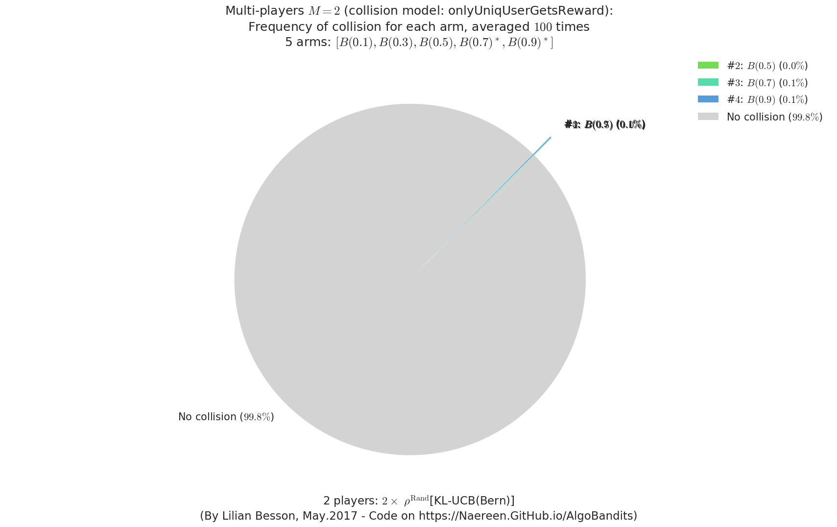
Final ranking for this environment #1 :
- Player #1, '#1<Selfish[KL-UCB(Bern)]>'  was ranked      1 / 2 for this simulation (last rewards = 7981.83).
- Player #2, '#2<Selfish[KL-UCB(Bern)]>'  was ranked      2 / 2 for this simulation (last rewards = 7861.44).
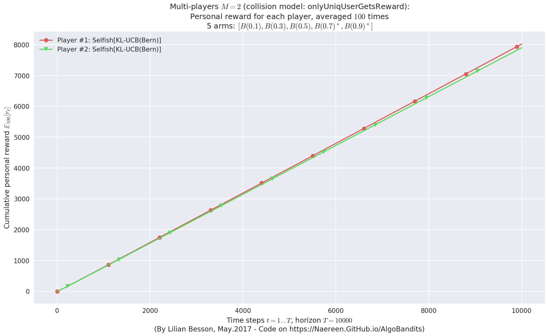
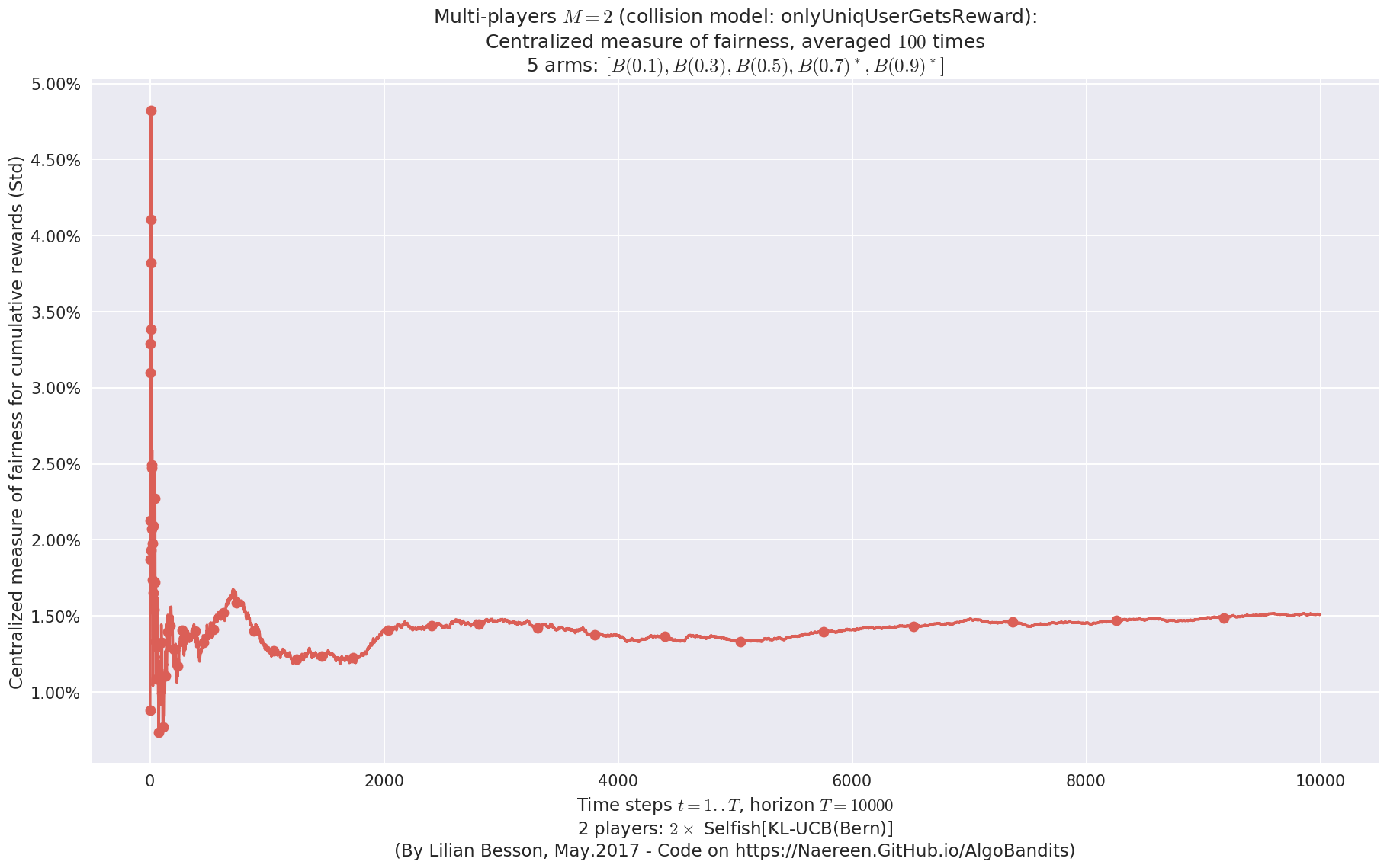
 -  For 2 players, Anandtharam et al. centralized lower-bound gave = 4.23 ...
 -  For 2 players, our lower bound gave = 8.46 ...
 -  For 2 players, the initial lower bound in Theorem 6 from [Anandkumar et al., 2010] gave = 5.35 ...

This MAB problem has:
 - a [Lai & Robbins] complexity constant C(mu) = 3.12 for 1-player problem ...
 - a Optimal Arm Identification factor H_OI(mu) = 40.00% ...
 - [Anandtharam et al] centralized lowerbound = 8.46,
 - Our decentralized lowerbound = 5.35,
 - [Anandkumar et al] decentralized lowerbound = 4.23
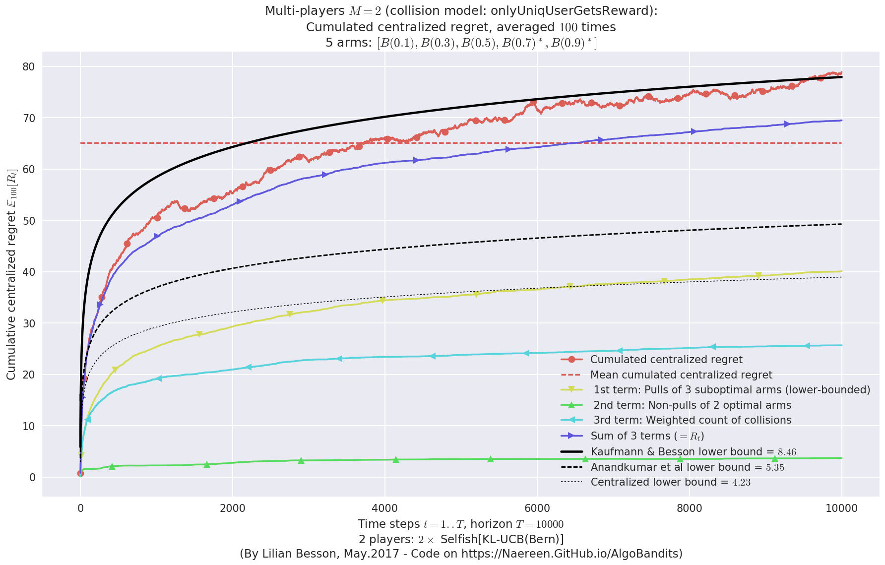
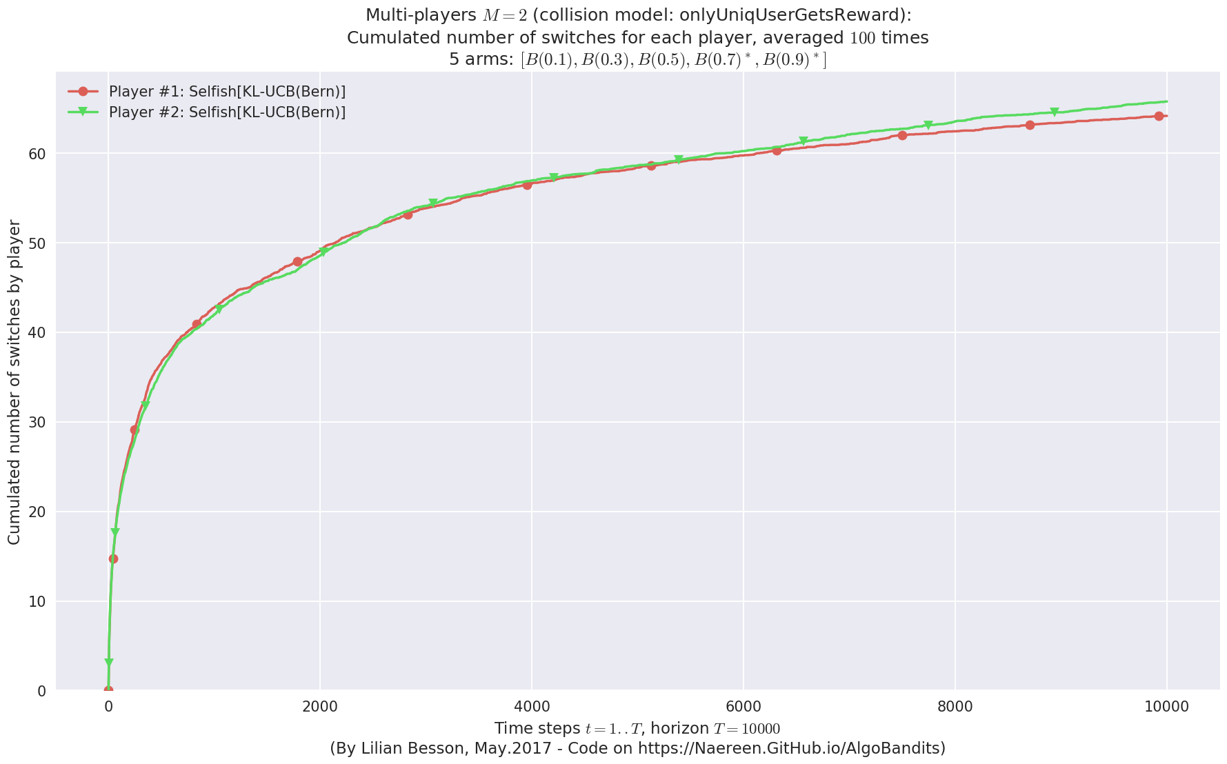
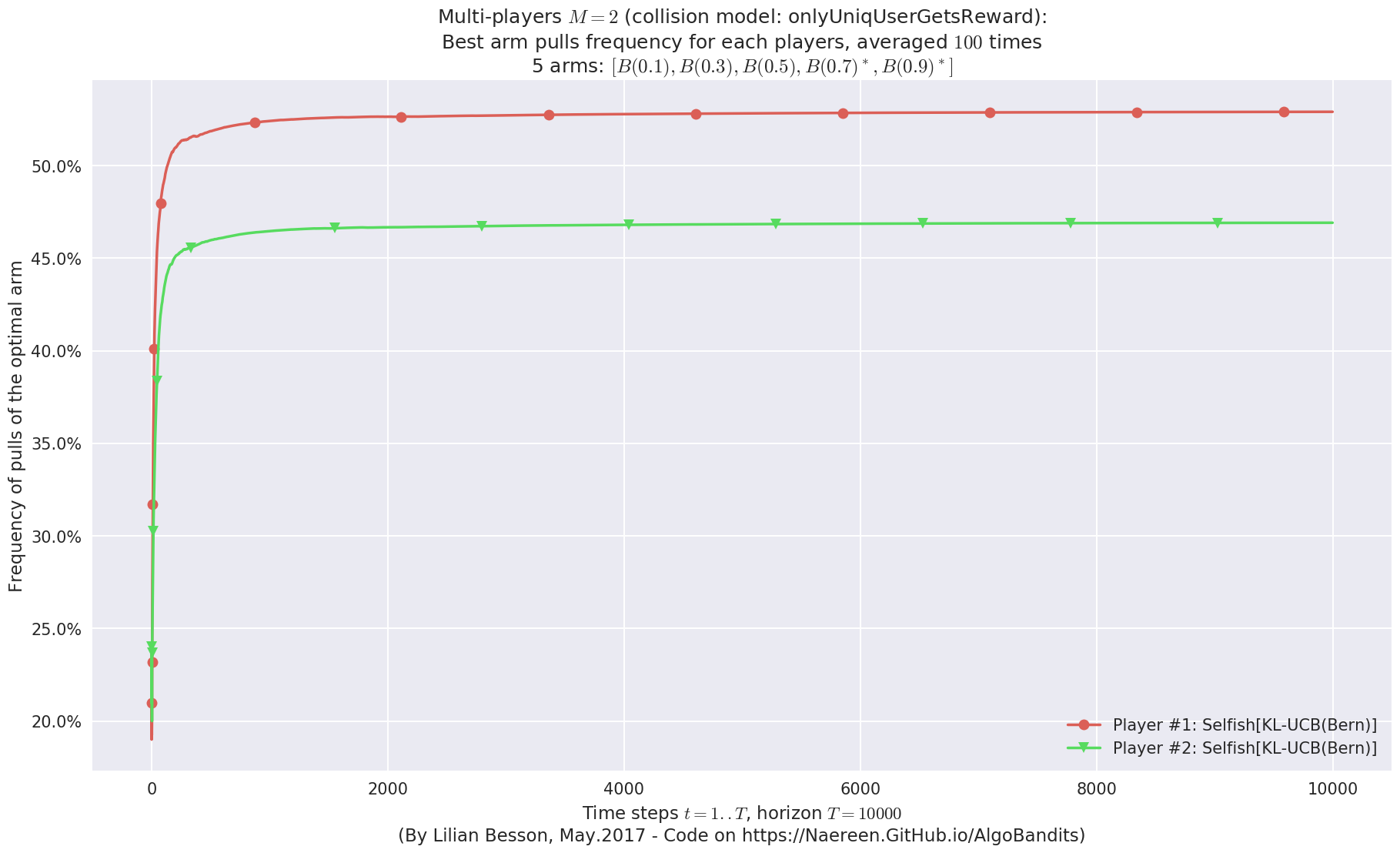
No upper bound for the non-cumulated number of collisions...
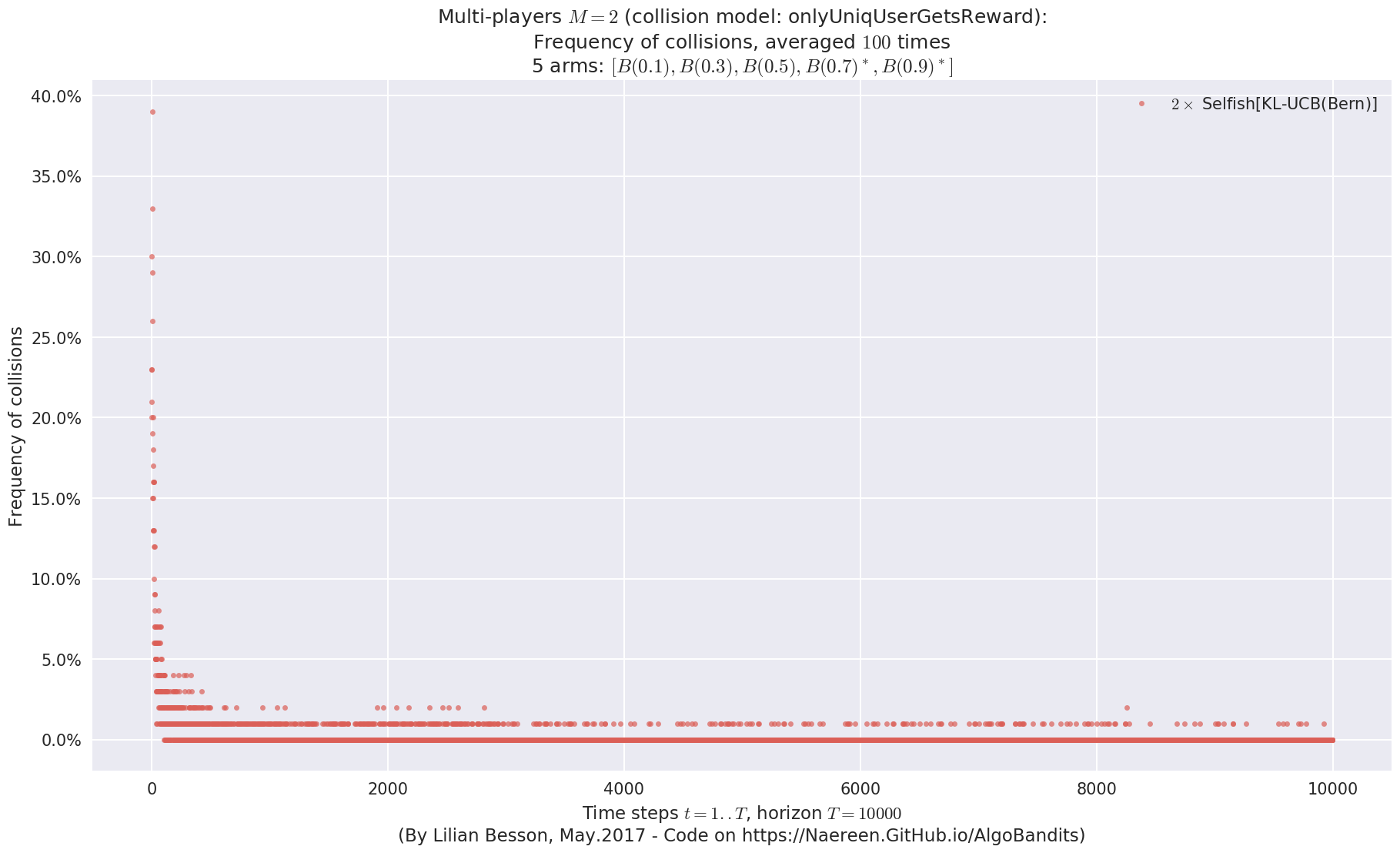
No upper bound for the non-cumulated number of collisions...

  - For #$0$: $B(0.1)$ ($0.0%$$\%$),    frequency of collisions is 3.5e-05  ...
  - For #$1$: $B(0.3)$ ($0.0%$$\%$),    frequency of collisions is 4.5e-05  ...
  - For #$2$: $B(0.5)$ ($0.0%$$\%$),    frequency of collisions is 9.5e-05  ...
  - For #$3$: $B(0.7)$ ($0.0%$$\%$),    frequency of collisions is 0.000402  ...
  - For #$4$: $B(0.9)$ ($0.1%$$\%$),    frequency of collisions is 0.001042  ...
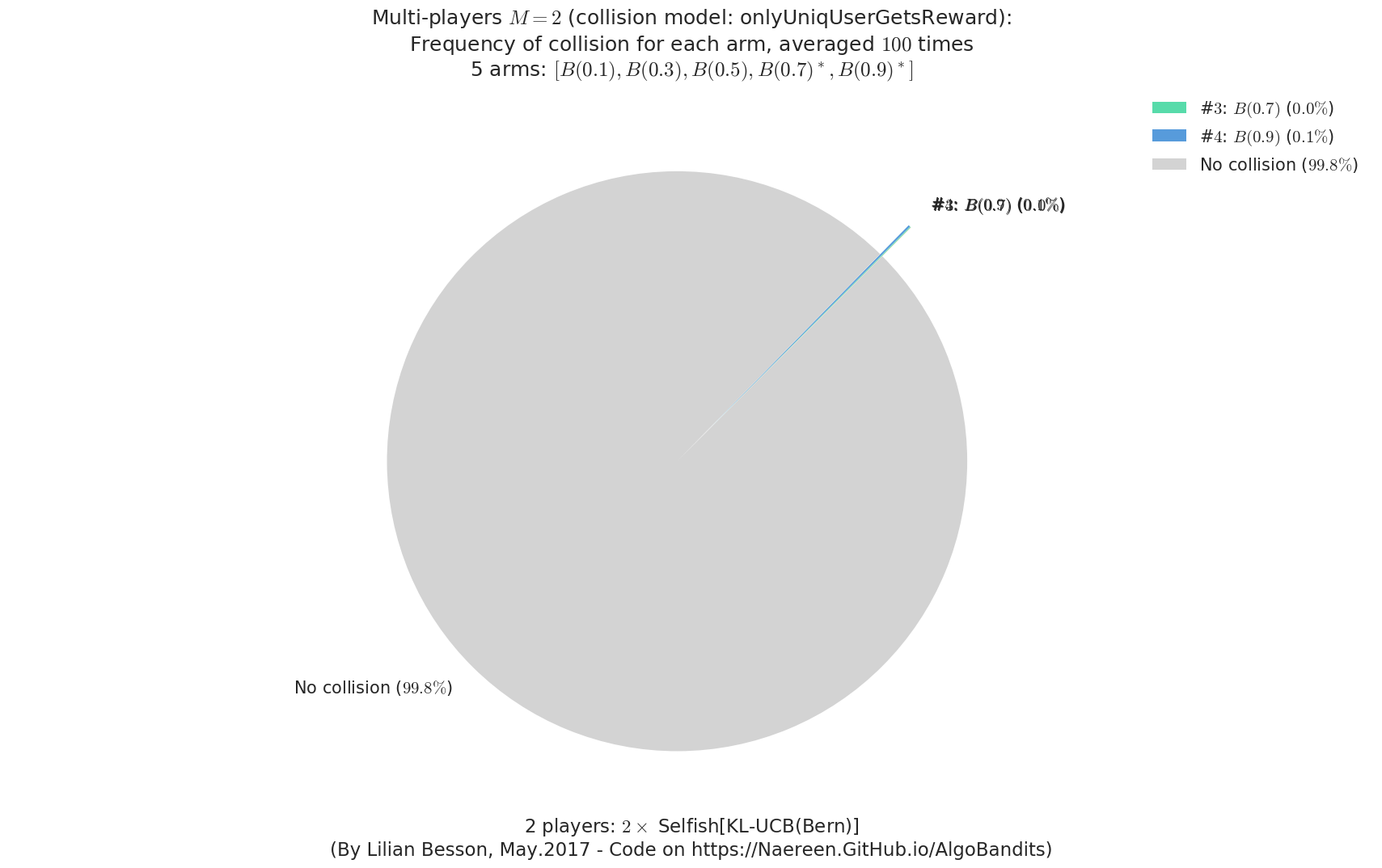
Third problem
\(\mu = [0.005, 0.01, 0.015, 0.84, 0.85]\) is an harder Bernoulli problem, as there is a huge gap between suboptimal and optimal arms.
In [27]:
for playersId in tqdm(range(len(evs)), desc="Policies"):
    evaluation = evaluators[2][playersId]
    plotAll(evaluation, 2)
Final ranking for this environment #2 :
- Player #1, '#1<$\rho^{\mathrm{Rand}}$[UCB($\alpha=1$)]>'        was ranked      1 / 2 for this simulation (last rewards = 8383.86).
- Player #2, '#2<$\rho^{\mathrm{Rand}}$[UCB($\alpha=1$)]>'        was ranked      2 / 2 for this simulation (last rewards = 8377.47).

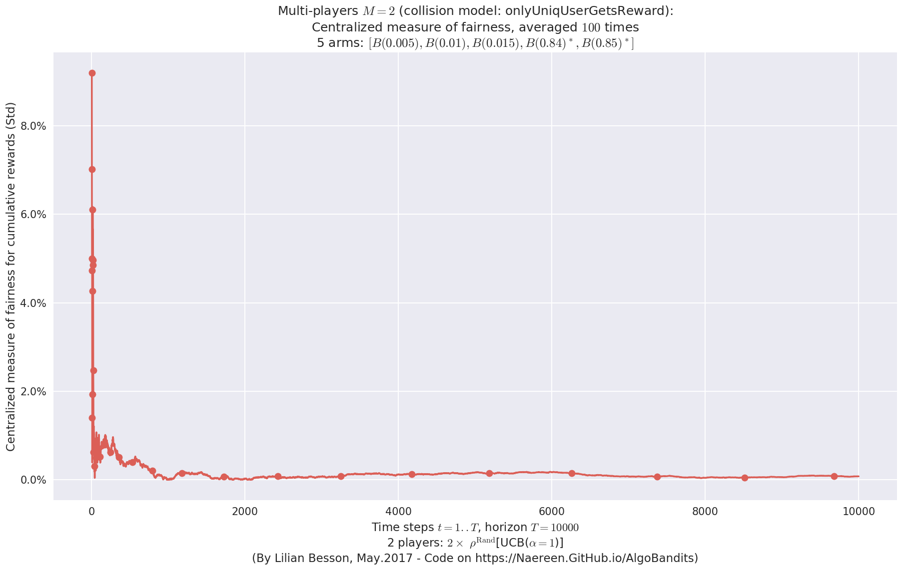
 -  For 2 players, Anandtharam et al. centralized lower-bound gave = 1.41 ...
 -  For 2 players, our lower bound gave = 2.83 ...
 -  For 2 players, the initial lower bound in Theorem 6 from [Anandkumar et al., 2010] gave = 2.78 ...

This MAB problem has:
 - a [Lai & Robbins] complexity constant C(mu) = 27.3 for 1-player problem ...
 - a Optimal Arm Identification factor H_OI(mu) = 29.40% ...
 - [Anandtharam et al] centralized lowerbound = 2.83,
 - Our decentralized lowerbound = 2.78,
 - [Anandkumar et al] decentralized lowerbound = 1.41
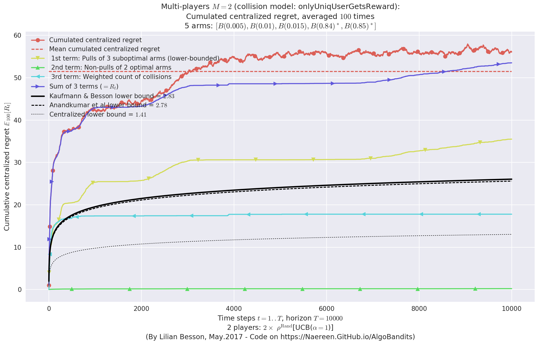
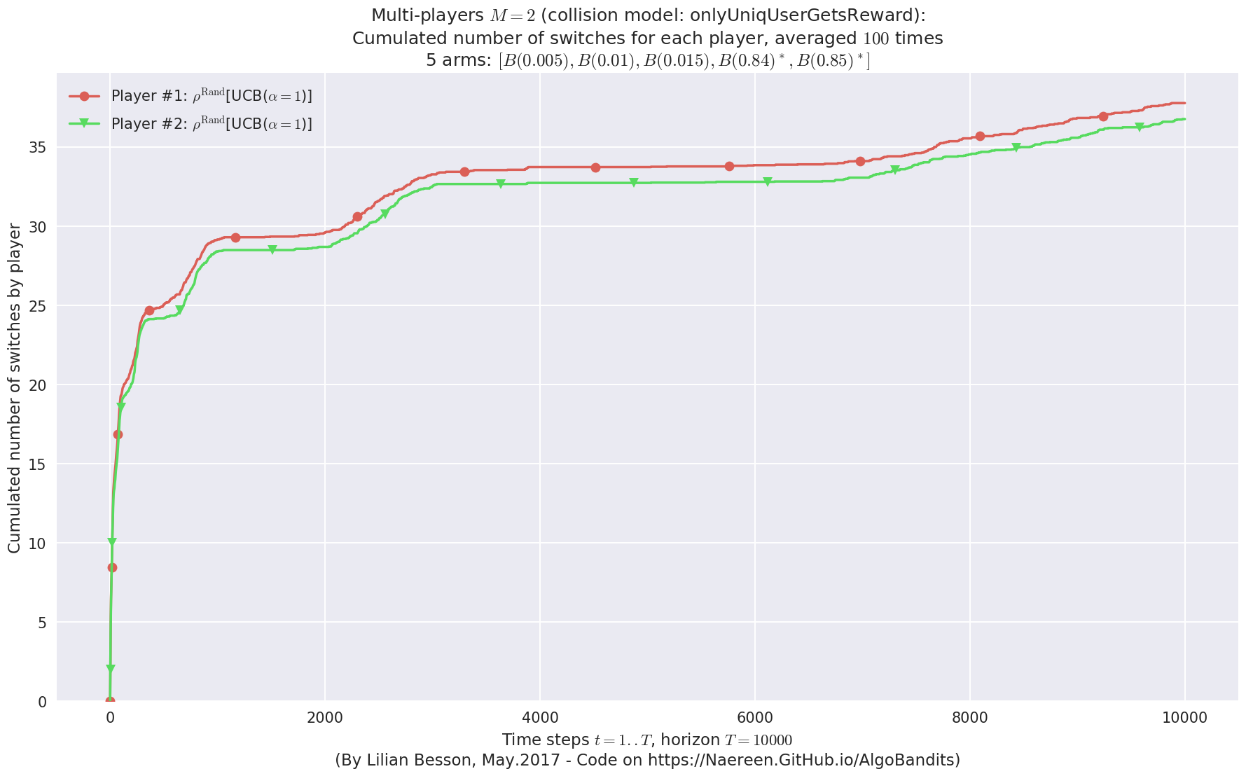
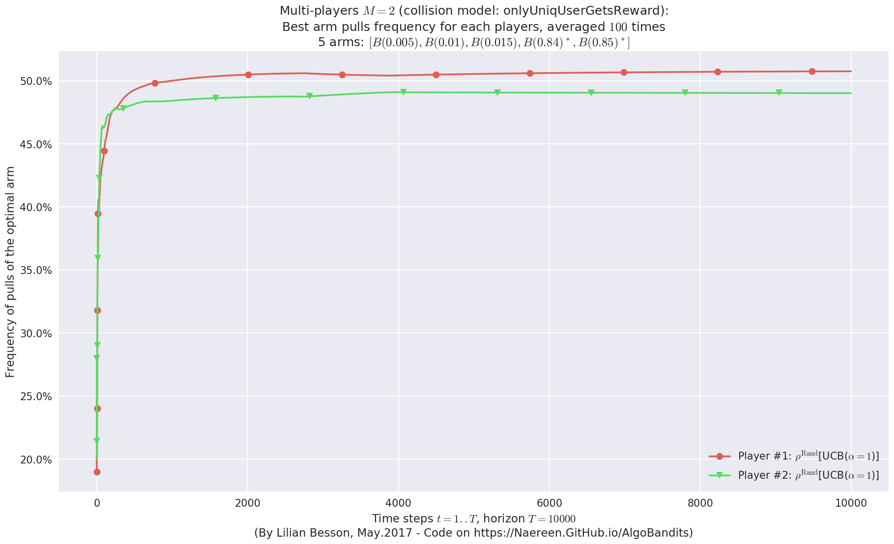
No upper bound for the non-cumulated number of collisions...
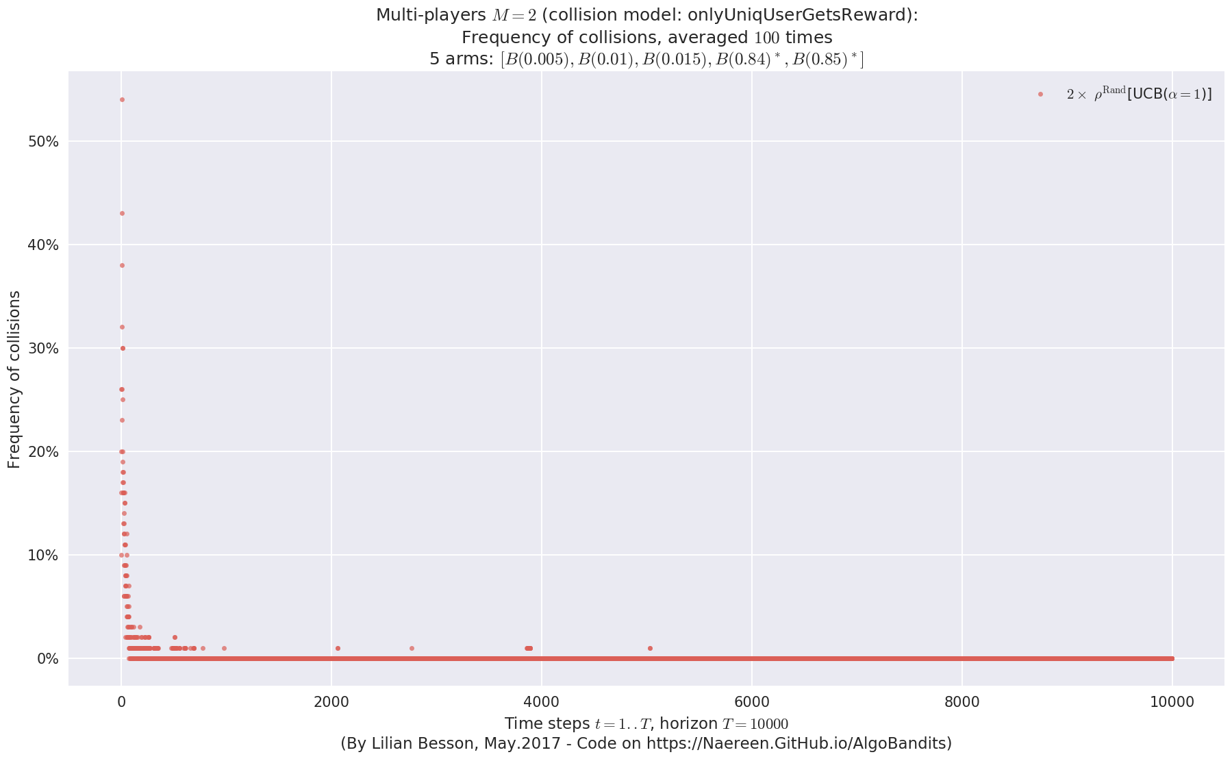
No upper bound for the non-cumulated number of collisions...
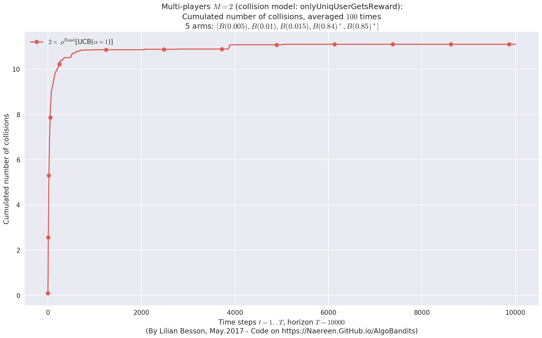
  - For #$0$: $B(0.005)$ ($0.0%$$\%$),  frequency of collisions is 1.7e-05  ...
  - For #$1$: $B(0.01)$ ($0.0%$$\%$),   frequency of collisions is 2.2e-05  ...
  - For #$2$: $B(0.015)$ ($0.0%$$\%$),  frequency of collisions is 1.9e-05  ...
  - For #$3$: $B(0.84)$ ($0.1%$$\%$),   frequency of collisions is 0.000546  ...
  - For #$4$: $B(0.85)$ ($0.1%$$\%$),   frequency of collisions is 0.000506  ...
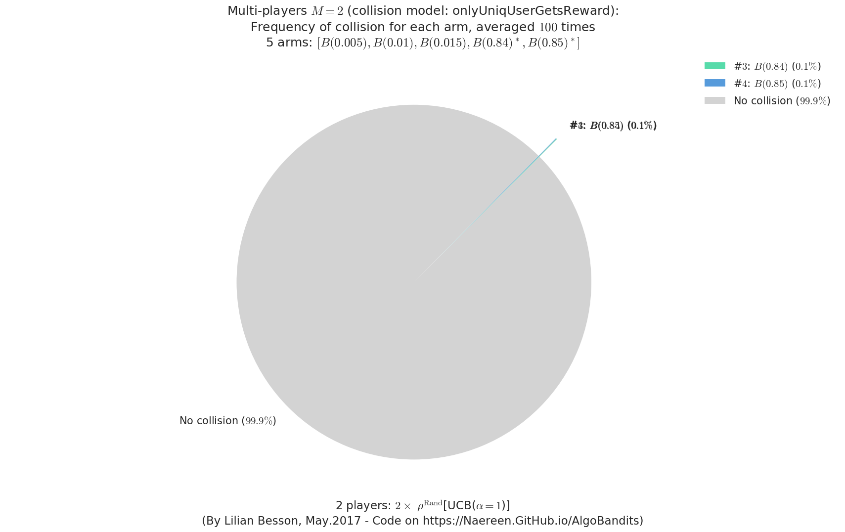
Final ranking for this environment #2 :
- Player #2, '#2<Selfish[UCB($\alpha=1$)]>'       was ranked      1 / 2 for this simulation (last rewards = 8377.35).
- Player #1, '#1<Selfish[UCB($\alpha=1$)]>'       was ranked      2 / 2 for this simulation (last rewards = 8369.71).

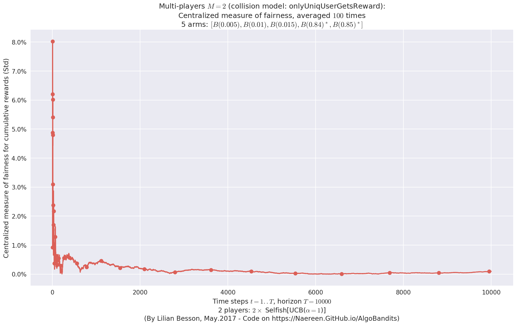
 -  For 2 players, Anandtharam et al. centralized lower-bound gave = 1.41 ...
 -  For 2 players, our lower bound gave = 2.83 ...
 -  For 2 players, the initial lower bound in Theorem 6 from [Anandkumar et al., 2010] gave = 2.78 ...

This MAB problem has:
 - a [Lai & Robbins] complexity constant C(mu) = 27.3 for 1-player problem ...
 - a Optimal Arm Identification factor H_OI(mu) = 29.40% ...
 - [Anandtharam et al] centralized lowerbound = 2.83,
 - Our decentralized lowerbound = 2.78,
 - [Anandkumar et al] decentralized lowerbound = 1.41
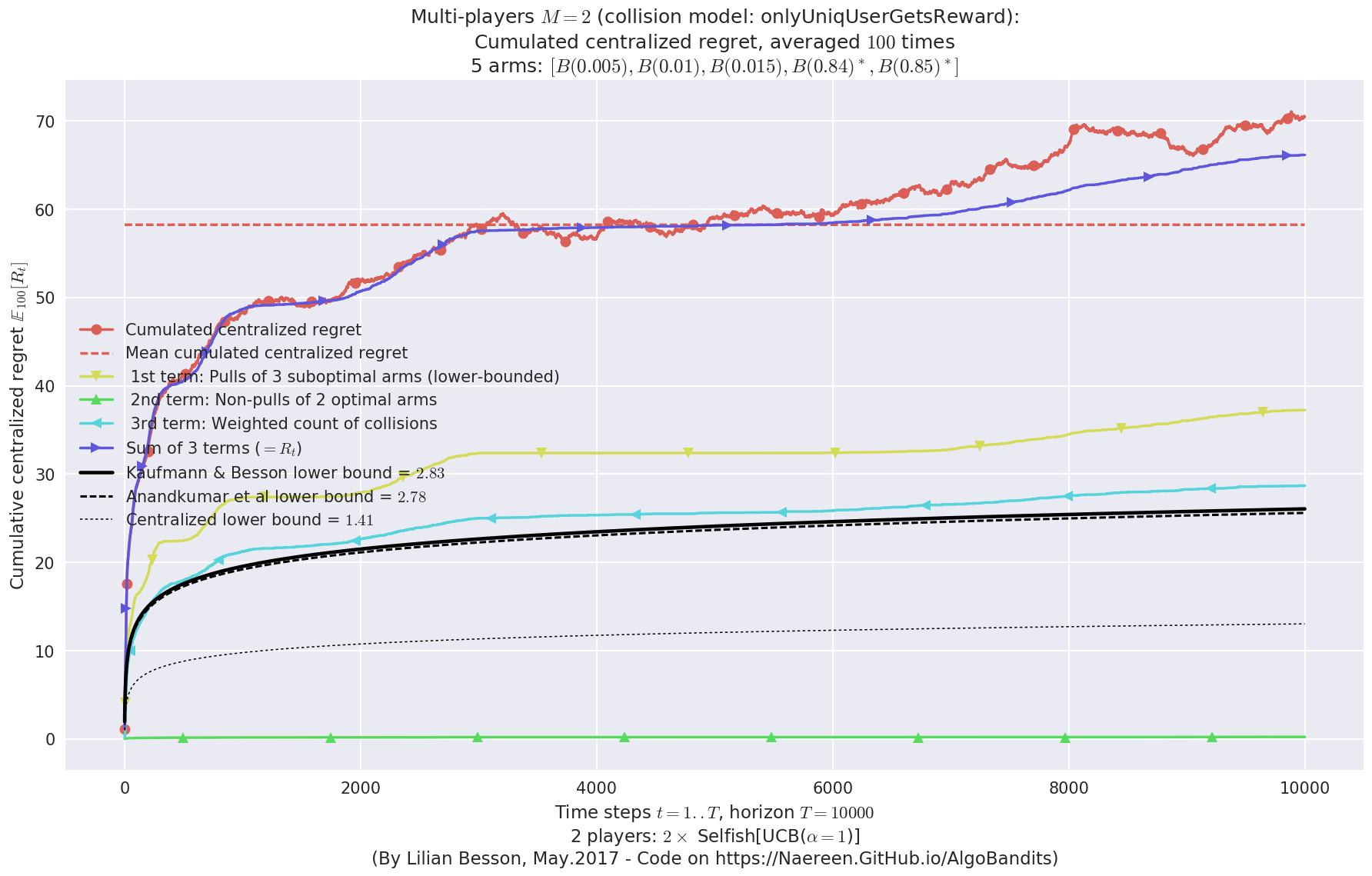
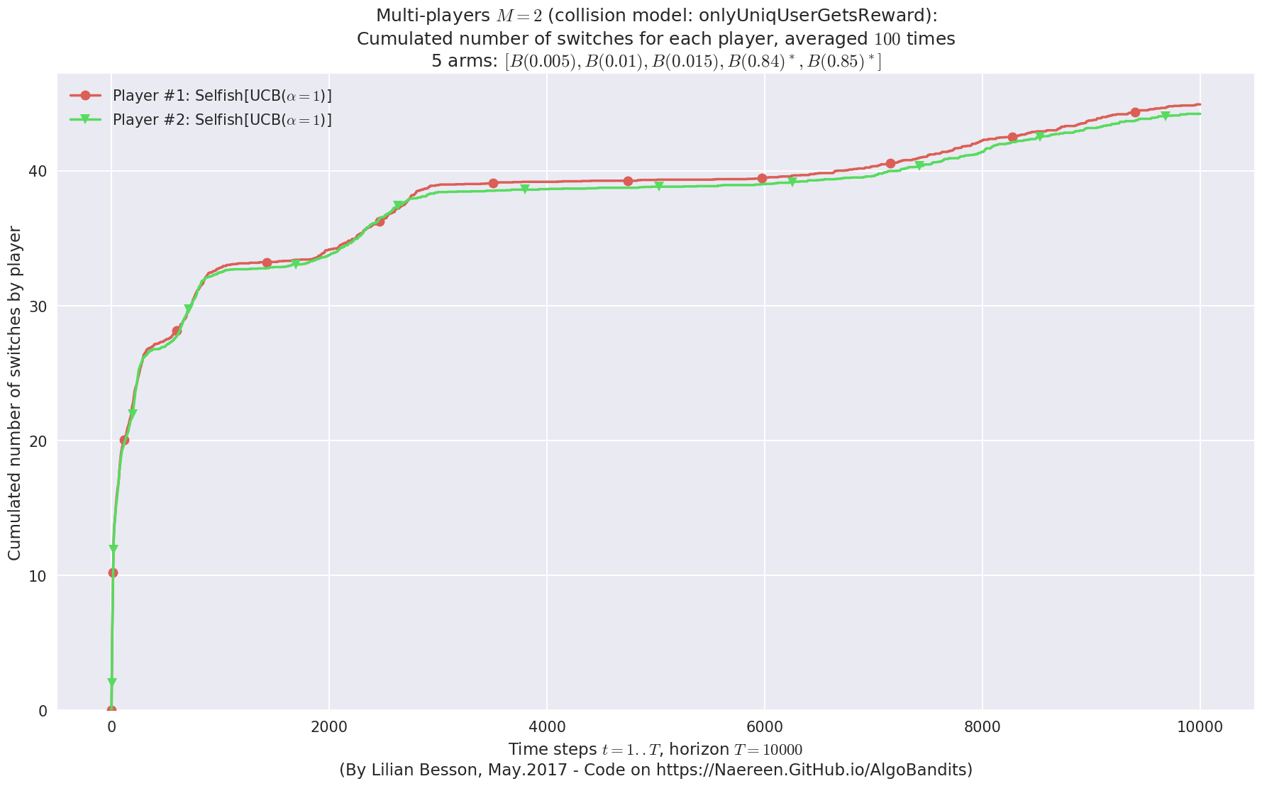
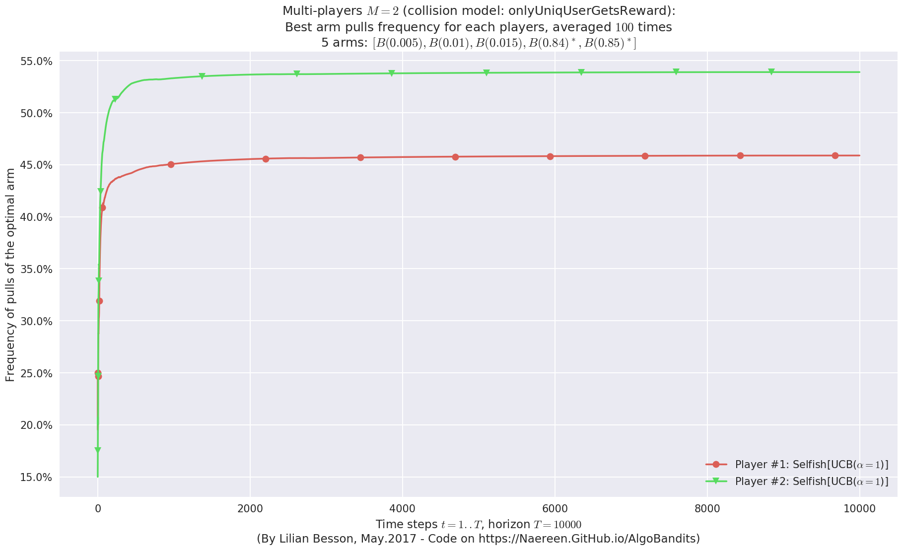
No upper bound for the non-cumulated number of collisions...
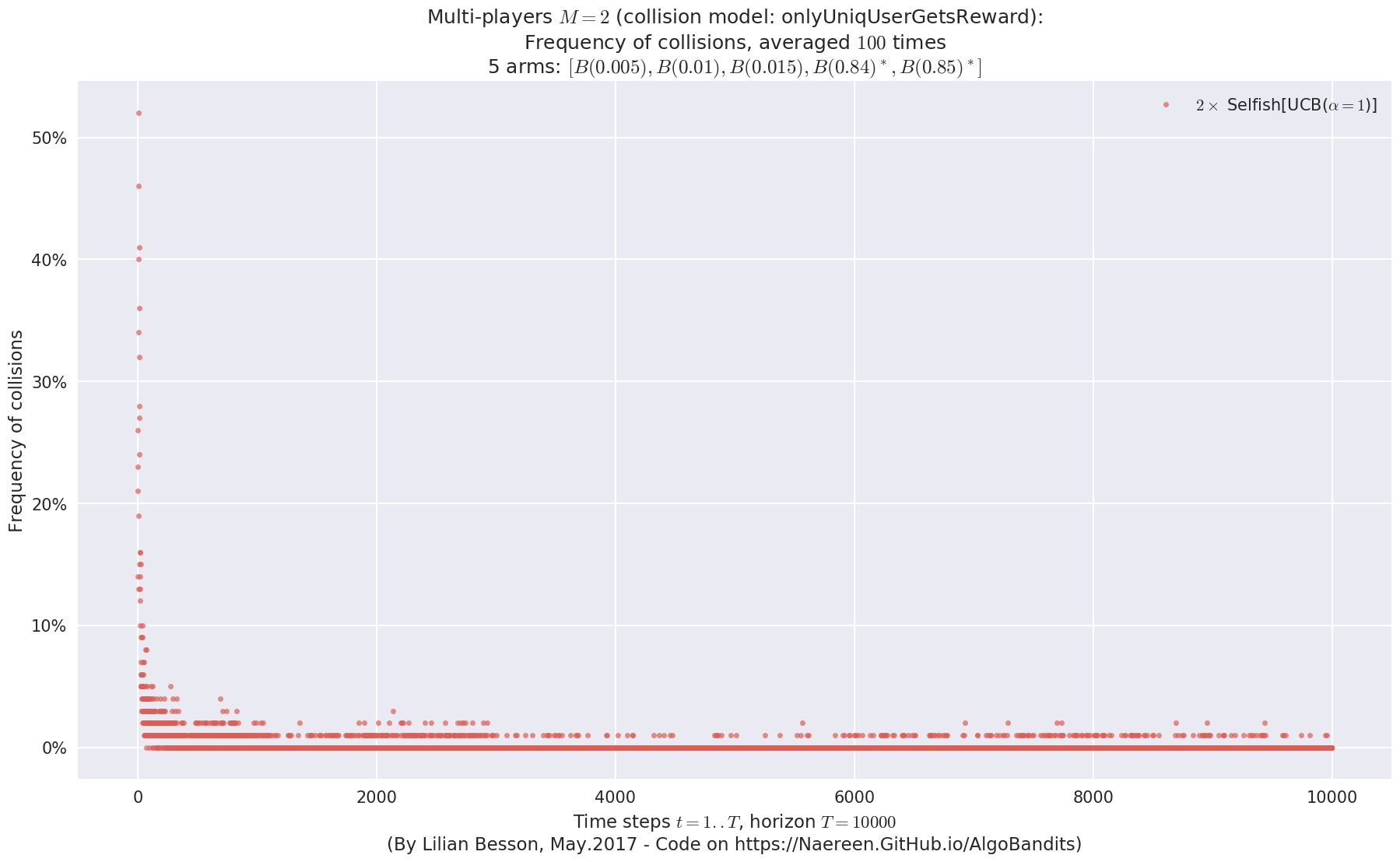
No upper bound for the non-cumulated number of collisions...

  - For #$0$: $B(0.005)$ ($0.0%$$\%$),  frequency of collisions is 5.8e-05  ...
  - For #$1$: $B(0.01)$ ($0.0%$$\%$),   frequency of collisions is 5.9e-05  ...
  - For #$2$: $B(0.015)$ ($0.0%$$\%$),  frequency of collisions is 5.2e-05  ...
  - For #$3$: $B(0.84)$ ($0.1%$$\%$),   frequency of collisions is 0.000833  ...
  - For #$4$: $B(0.85)$ ($0.1%$$\%$),   frequency of collisions is 0.000862  ...
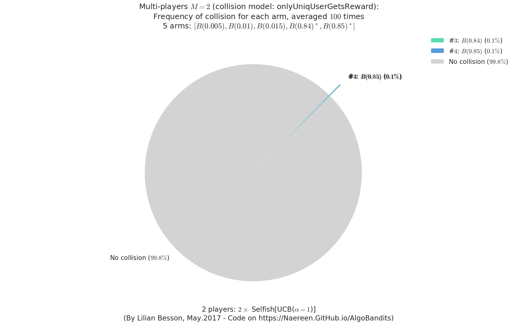
Final ranking for this environment #2 :
- Player #1, '#1<$\rho^{\mathrm{Rand}}$[Thompson]>'       was ranked      1 / 2 for this simulation (last rewards = 5303.43).
- Player #2, '#2<$\rho^{\mathrm{Rand}}$[Thompson]>'       was ranked      2 / 2 for this simulation (last rewards = 5301).

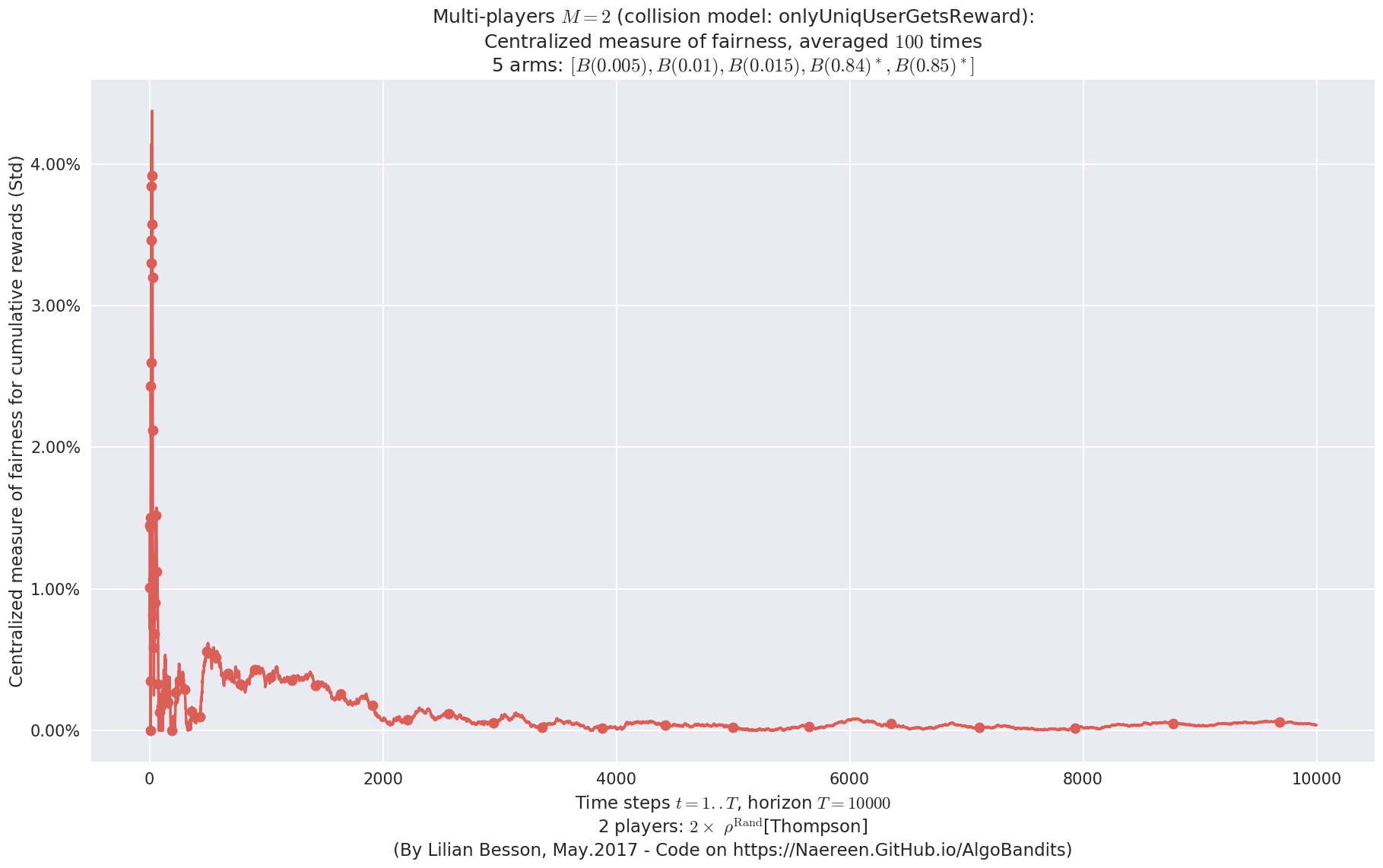
 -  For 2 players, Anandtharam et al. centralized lower-bound gave = 1.41 ...
 -  For 2 players, our lower bound gave = 2.83 ...
 -  For 2 players, the initial lower bound in Theorem 6 from [Anandkumar et al., 2010] gave = 2.78 ...

This MAB problem has:
 - a [Lai & Robbins] complexity constant C(mu) = 27.3 for 1-player problem ...
 - a Optimal Arm Identification factor H_OI(mu) = 29.40% ...
 - [Anandtharam et al] centralized lowerbound = 2.83,
 - Our decentralized lowerbound = 2.78,
 - [Anandkumar et al] decentralized lowerbound = 1.41
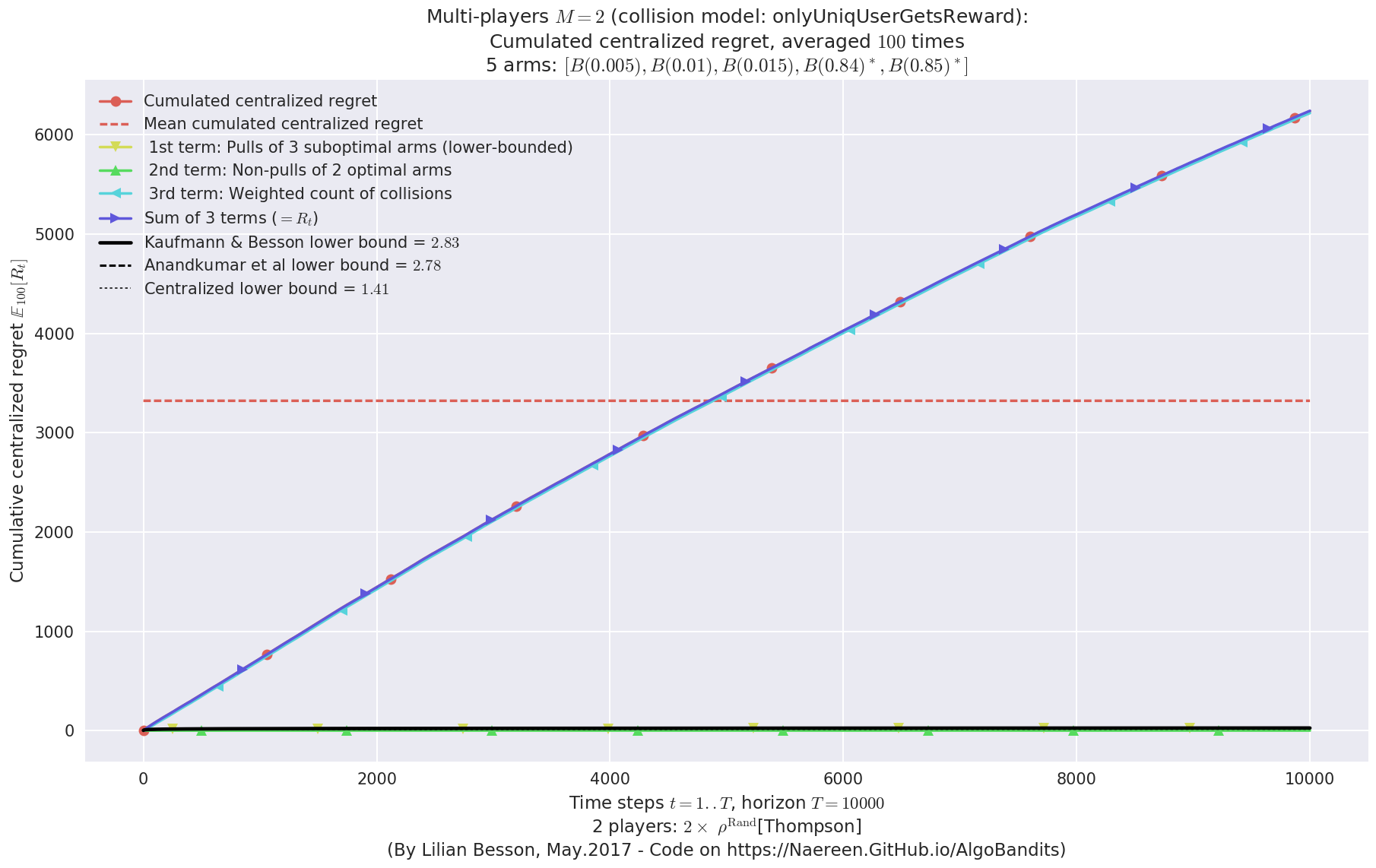
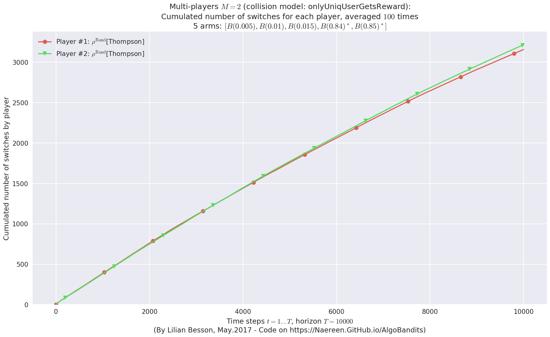
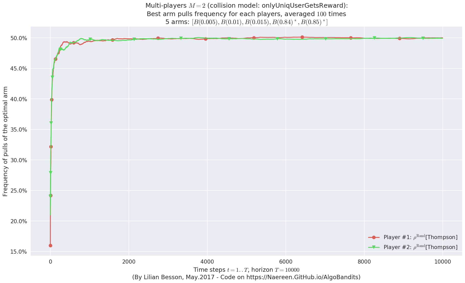
No upper bound for the non-cumulated number of collisions...
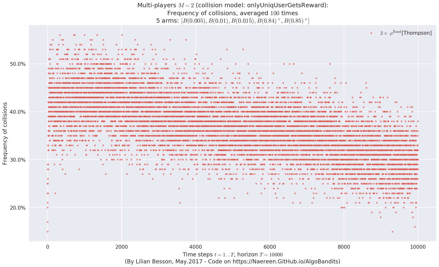
No upper bound for the non-cumulated number of collisions...
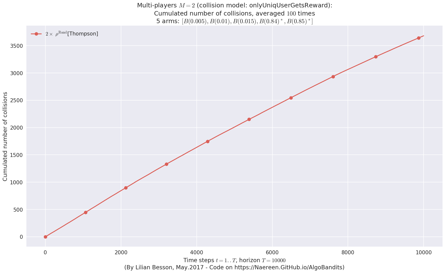
  - For #$0$: $B(0.005)$ ($0.0%$$\%$),  frequency of collisions is 3.1e-05  ...
  - For #$1$: $B(0.01)$ ($0.0%$$\%$),   frequency of collisions is 3.2e-05  ...
  - For #$2$: $B(0.015)$ ($0.0%$$\%$),  frequency of collisions is 3.6e-05  ...
  - For #$3$: $B(0.84)$ ($18.4%$$\%$),  frequency of collisions is 0.183667  ...
  - For #$4$: $B(0.85)$ ($18.4%$$\%$),  frequency of collisions is 0.184274  ...
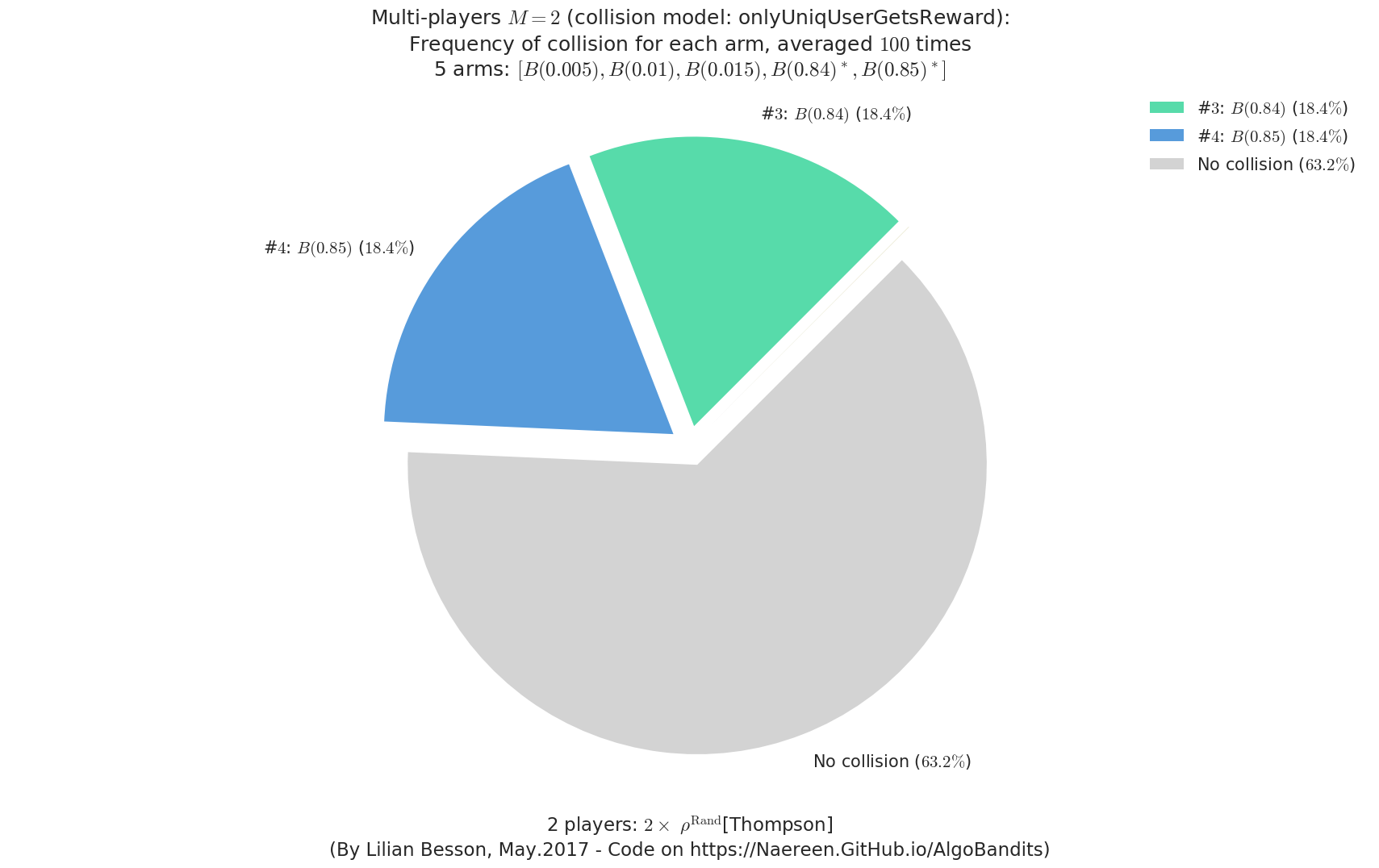
Final ranking for this environment #2 :
- Player #1, '#1<Selfish[Thompson]>'      was ranked      1 / 2 for this simulation (last rewards = 8393.01).
- Player #2, '#2<Selfish[Thompson]>'      was ranked      2 / 2 for this simulation (last rewards = 8388.5).
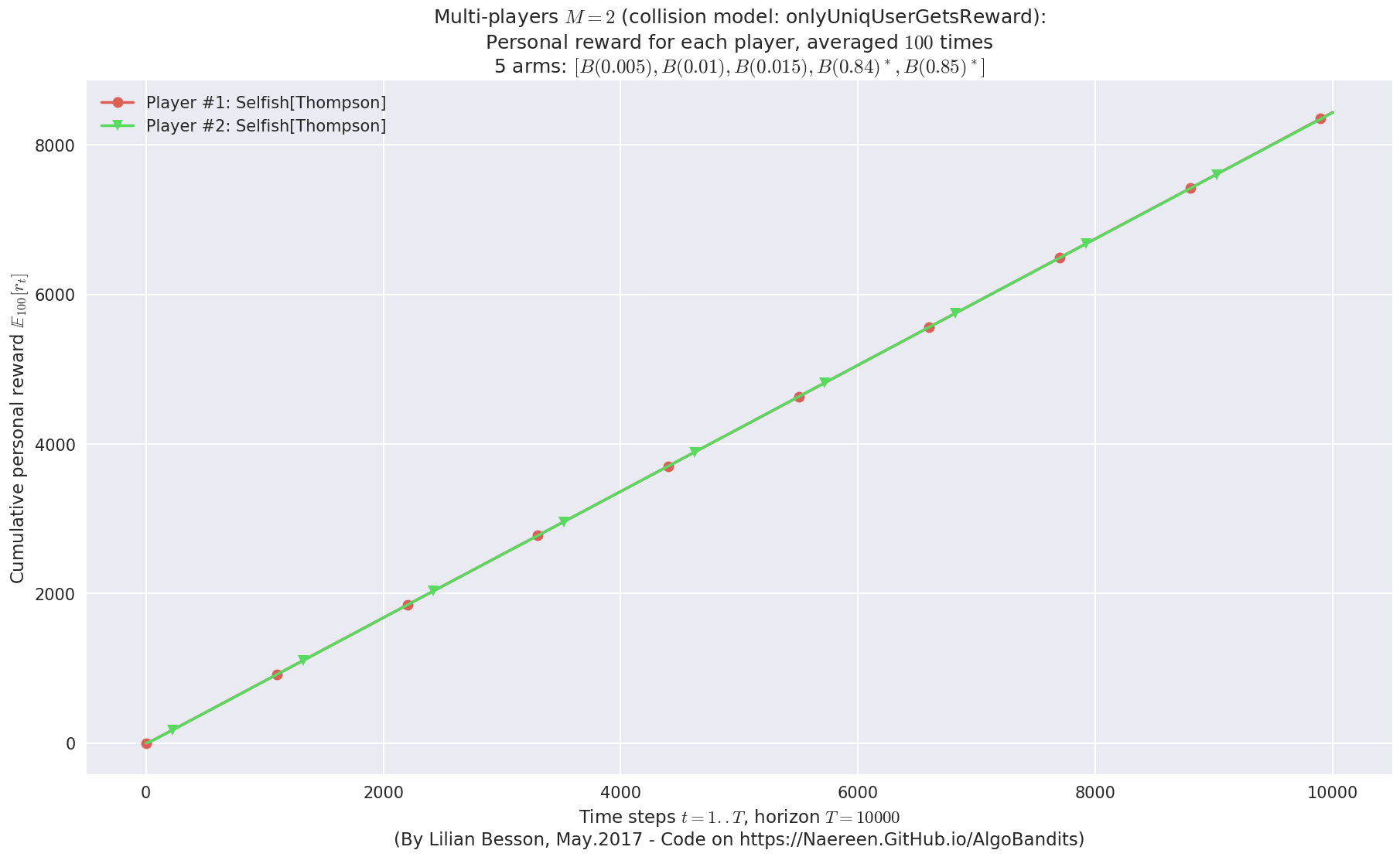
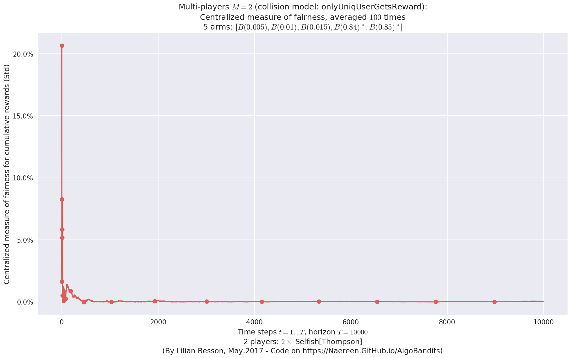
 -  For 2 players, Anandtharam et al. centralized lower-bound gave = 1.41 ...
 -  For 2 players, our lower bound gave = 2.83 ...
 -  For 2 players, the initial lower bound in Theorem 6 from [Anandkumar et al., 2010] gave = 2.78 ...

This MAB problem has:
 - a [Lai & Robbins] complexity constant C(mu) = 27.3 for 1-player problem ...
 - a Optimal Arm Identification factor H_OI(mu) = 29.40% ...
 - [Anandtharam et al] centralized lowerbound = 2.83,
 - Our decentralized lowerbound = 2.78,
 - [Anandkumar et al] decentralized lowerbound = 1.41
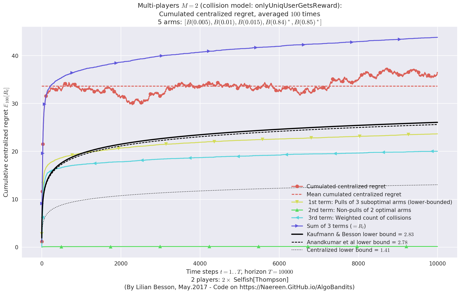
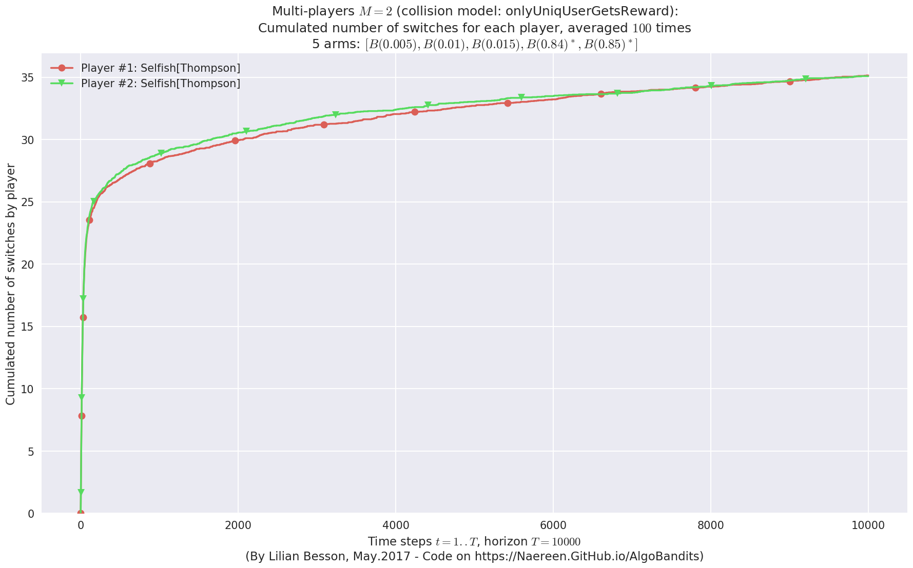
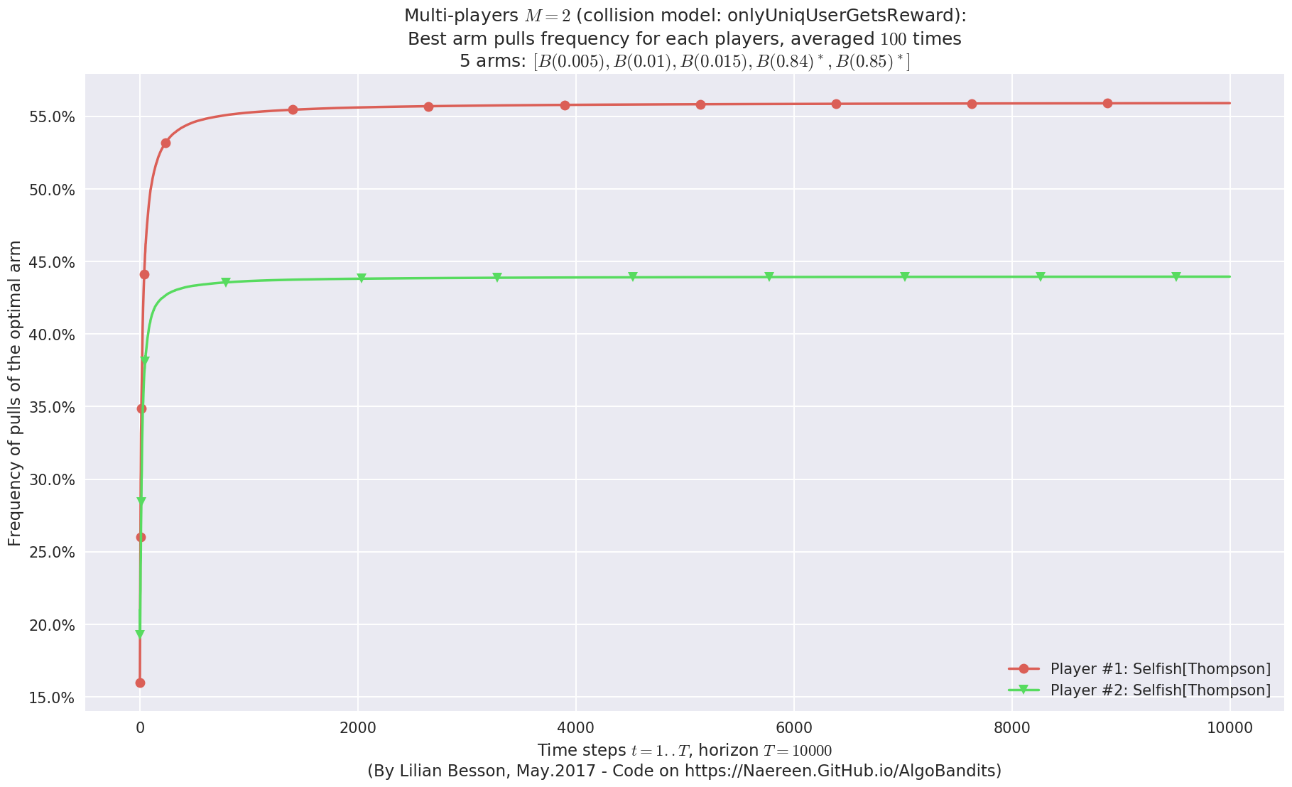
No upper bound for the non-cumulated number of collisions...
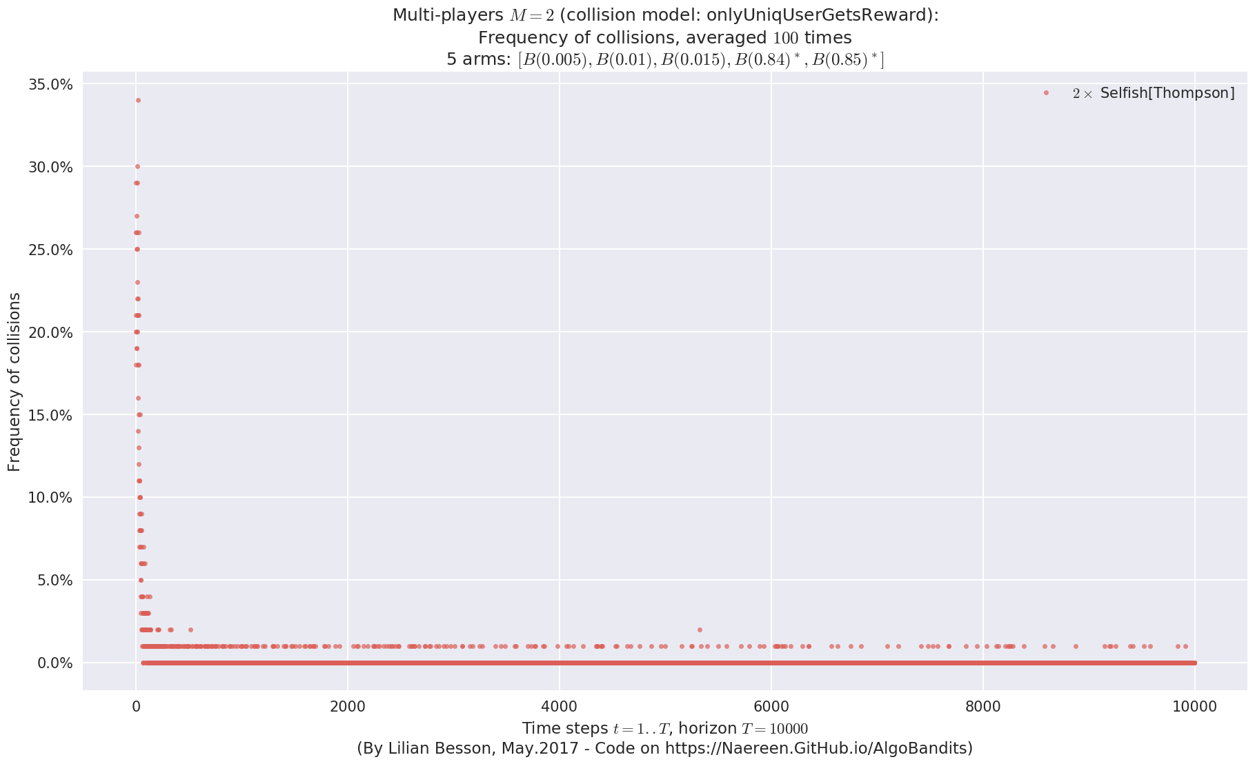
No upper bound for the non-cumulated number of collisions...
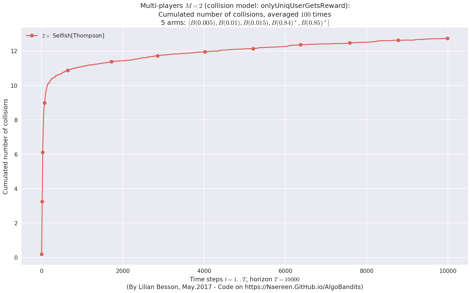
  - For #$0$: $B(0.005)$ ($0.0%$$\%$),  frequency of collisions is 3.1e-05  ...
  - For #$1$: $B(0.01)$ ($0.0%$$\%$),   frequency of collisions is 3.1e-05  ...
  - For #$2$: $B(0.015)$ ($0.0%$$\%$),  frequency of collisions is 2.8e-05  ...
  - For #$3$: $B(0.84)$ ($0.1%$$\%$),   frequency of collisions is 0.000573  ...
  - For #$4$: $B(0.85)$ ($0.1%$$\%$),   frequency of collisions is 0.00061  ...

Final ranking for this environment #2 :
- Player #1, '#1<$\rho^{\mathrm{Rand}}$[KL-UCB(Bern)]>'   was ranked      1 / 2 for this simulation (last rewards = 8385.77).
- Player #2, '#2<$\rho^{\mathrm{Rand}}$[KL-UCB(Bern)]>'   was ranked      2 / 2 for this simulation (last rewards = 8376.99).
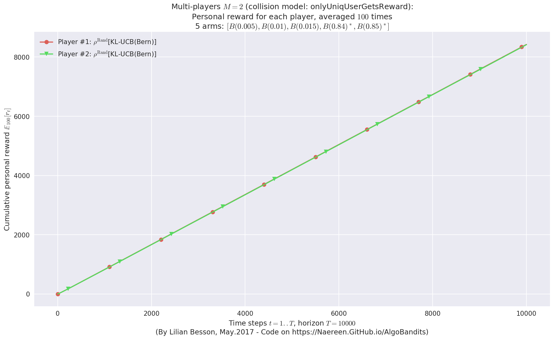
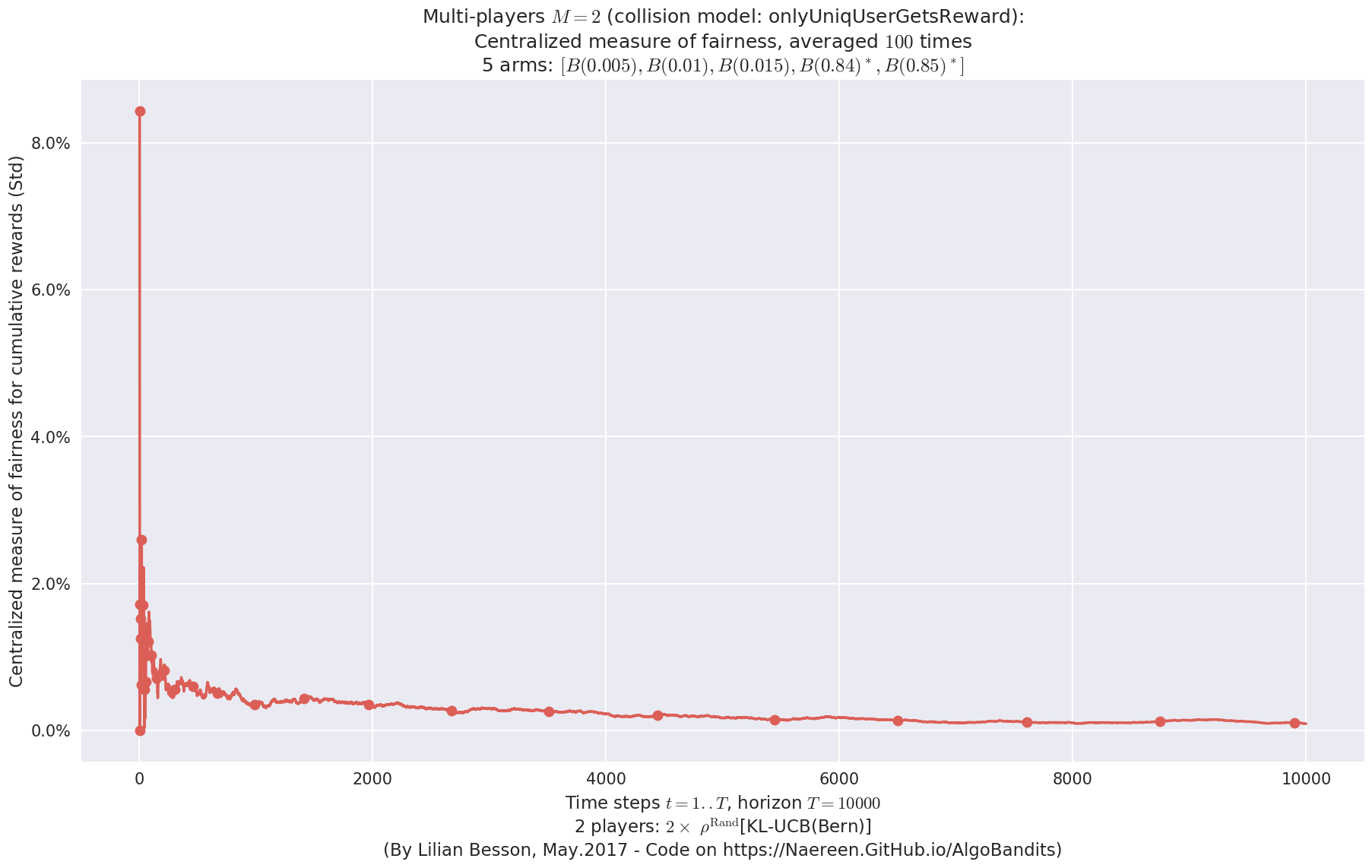
 -  For 2 players, Anandtharam et al. centralized lower-bound gave = 1.41 ...
 -  For 2 players, our lower bound gave = 2.83 ...
 -  For 2 players, the initial lower bound in Theorem 6 from [Anandkumar et al., 2010] gave = 2.78 ...

This MAB problem has:
 - a [Lai & Robbins] complexity constant C(mu) = 27.3 for 1-player problem ...
 - a Optimal Arm Identification factor H_OI(mu) = 29.40% ...
 - [Anandtharam et al] centralized lowerbound = 2.83,
 - Our decentralized lowerbound = 2.78,
 - [Anandkumar et al] decentralized lowerbound = 1.41
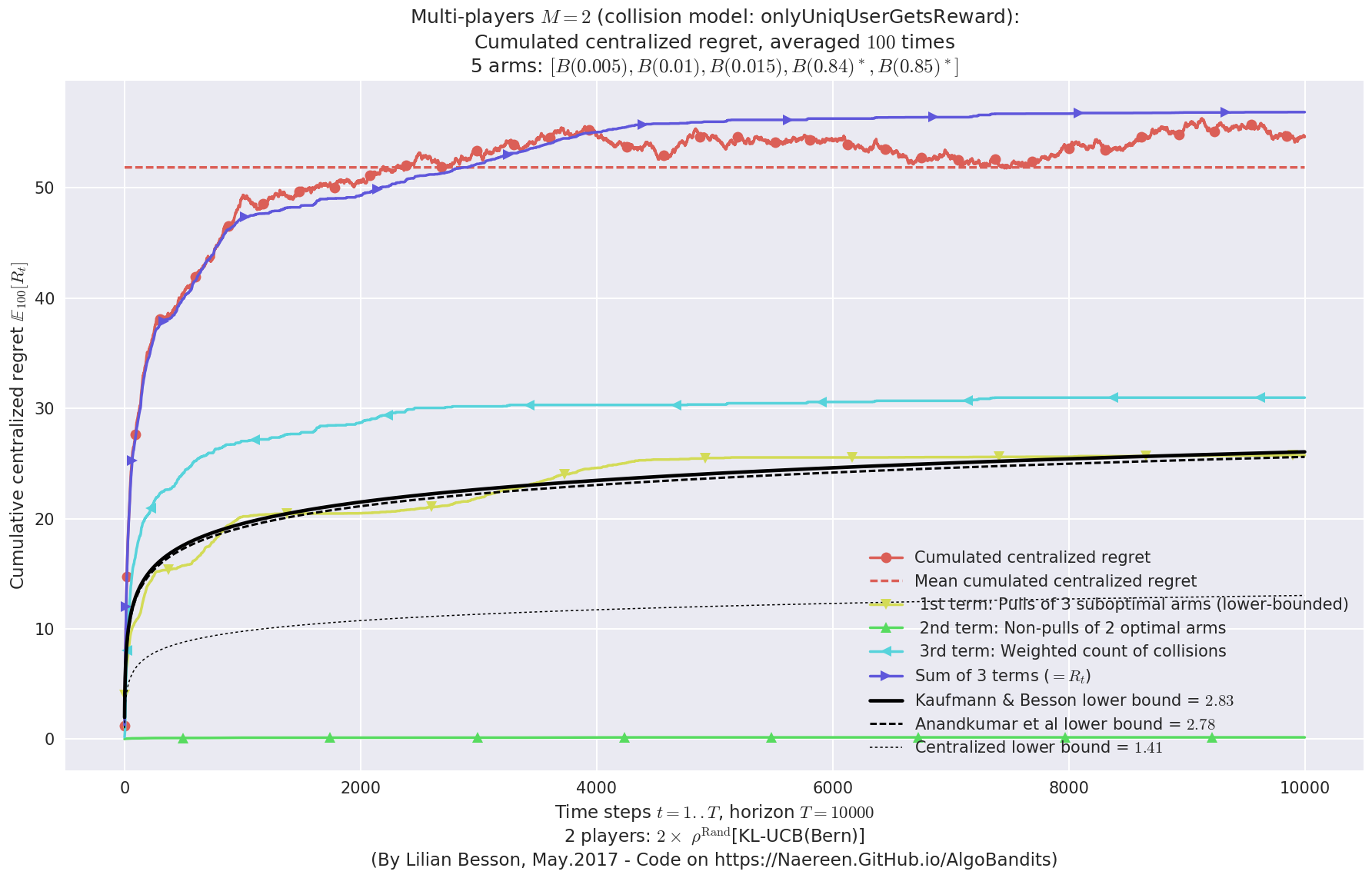
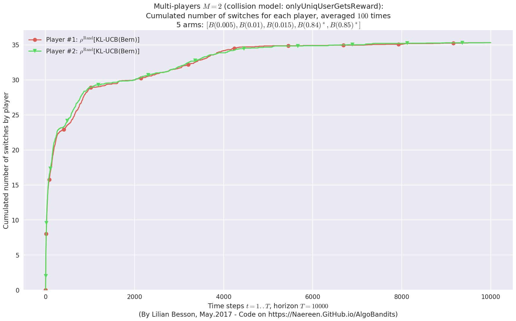
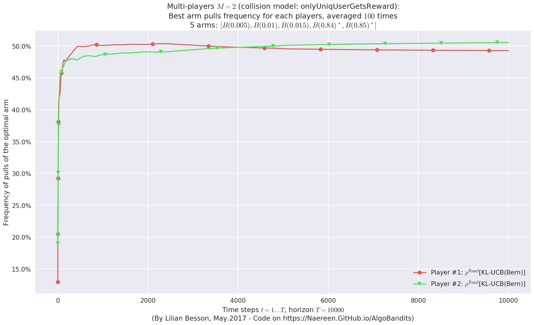
No upper bound for the non-cumulated number of collisions...
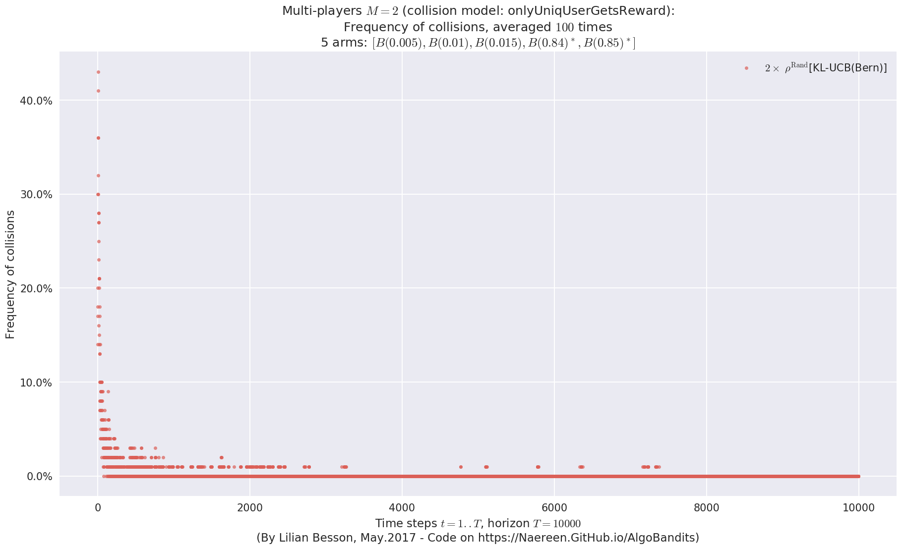
No upper bound for the non-cumulated number of collisions...
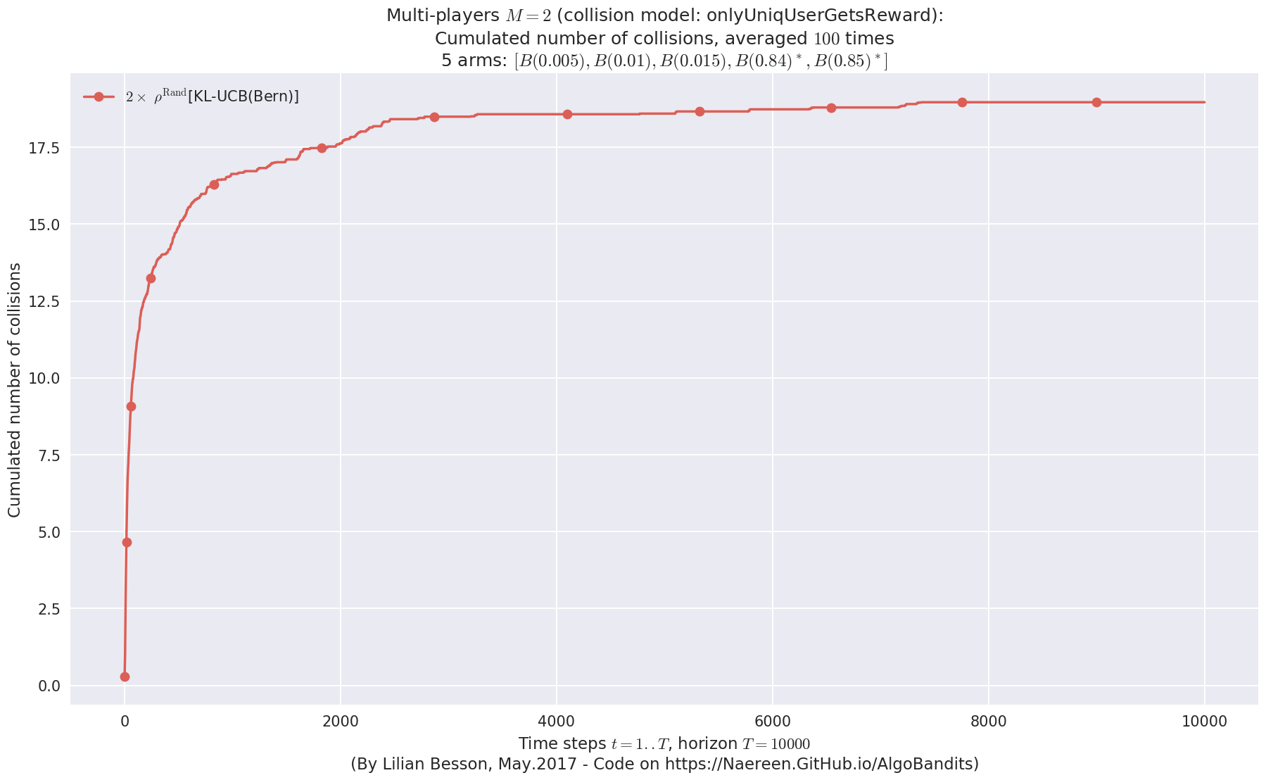
  - For #$0$: $B(0.005)$ ($0.0%$$\%$),  frequency of collisions is 1.8e-05  ...
  - For #$1$: $B(0.01)$ ($0.0%$$\%$),   frequency of collisions is 2.2e-05  ...
  - For #$2$: $B(0.015)$ ($0.0%$$\%$),  frequency of collisions is 2.4e-05  ...
  - For #$3$: $B(0.84)$ ($0.1%$$\%$),   frequency of collisions is 0.000934  ...
  - For #$4$: $B(0.85)$ ($0.1%$$\%$),   frequency of collisions is 0.000898  ...

Final ranking for this environment #2 :
- Player #2, '#2<Selfish[KL-UCB(Bern)]>'  was ranked      1 / 2 for this simulation (last rewards = 8386.17).
- Player #1, '#1<Selfish[KL-UCB(Bern)]>'  was ranked      2 / 2 for this simulation (last rewards = 8382.05).
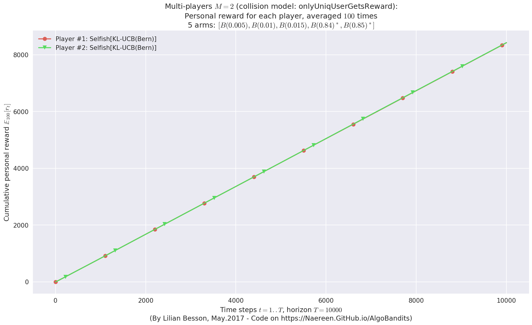
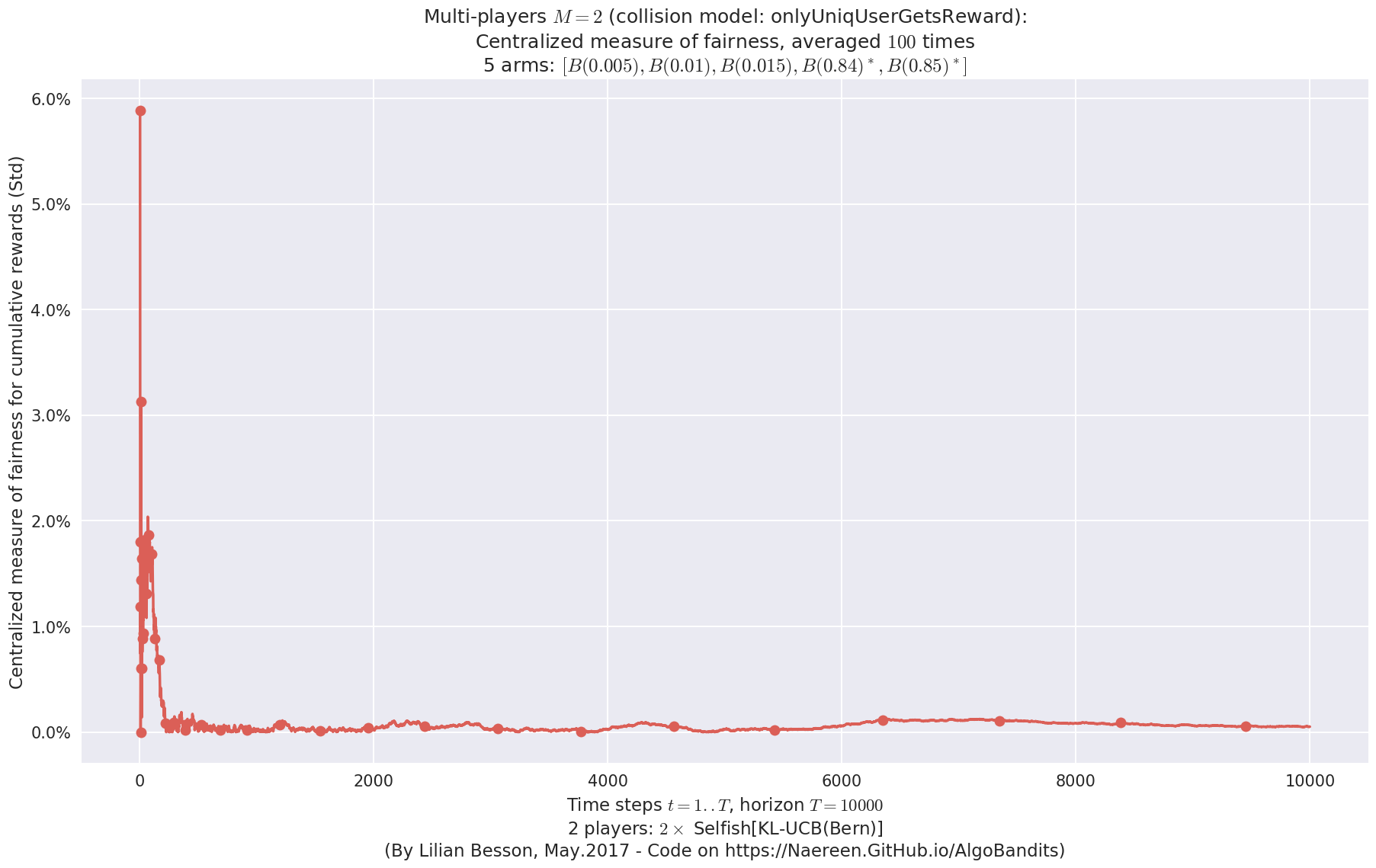
 -  For 2 players, Anandtharam et al. centralized lower-bound gave = 1.41 ...
 -  For 2 players, our lower bound gave = 2.83 ...
 -  For 2 players, the initial lower bound in Theorem 6 from [Anandkumar et al., 2010] gave = 2.78 ...

This MAB problem has:
 - a [Lai & Robbins] complexity constant C(mu) = 27.3 for 1-player problem ...
 - a Optimal Arm Identification factor H_OI(mu) = 29.40% ...
 - [Anandtharam et al] centralized lowerbound = 2.83,
 - Our decentralized lowerbound = 2.78,
 - [Anandkumar et al] decentralized lowerbound = 1.41
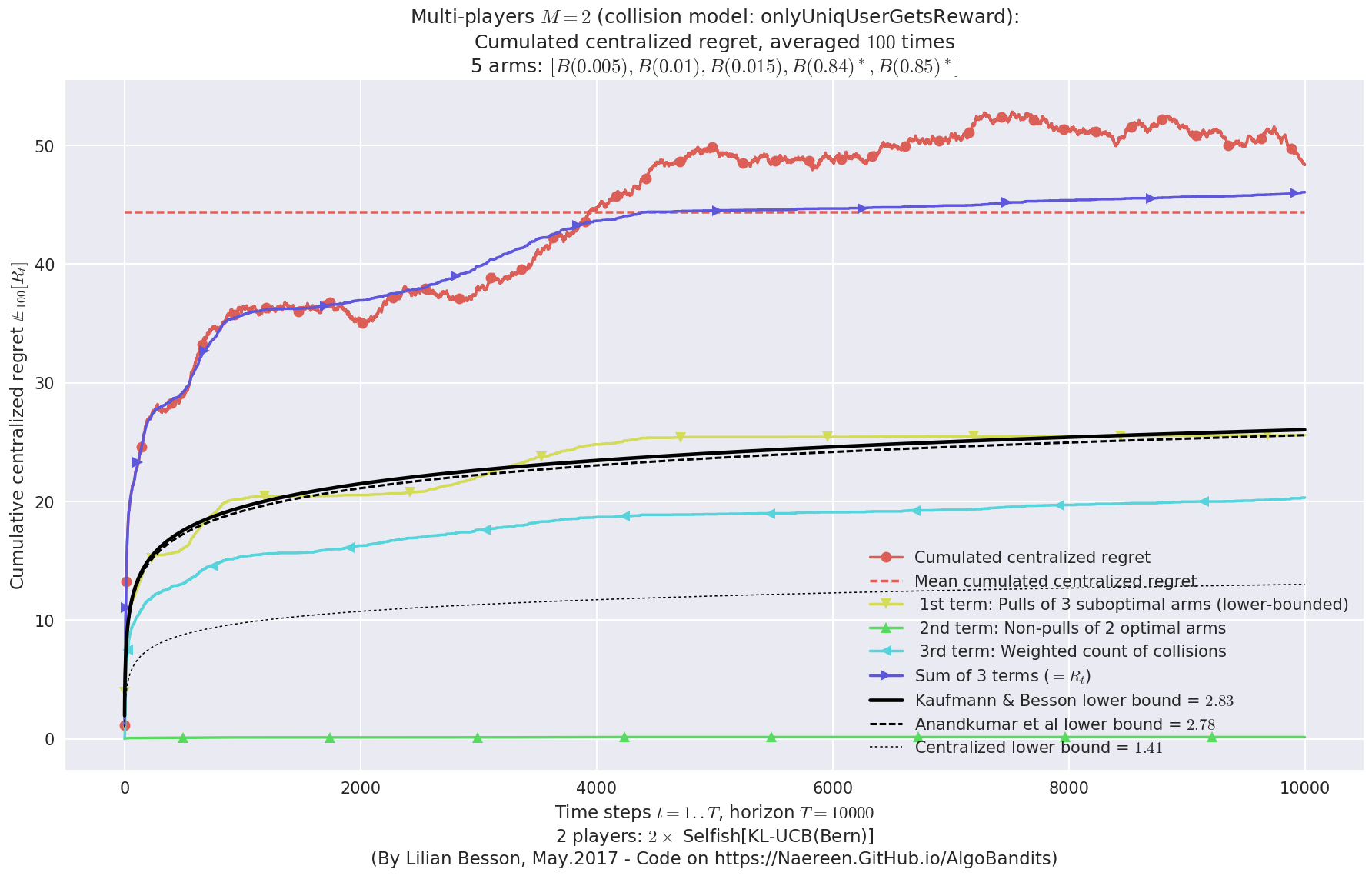
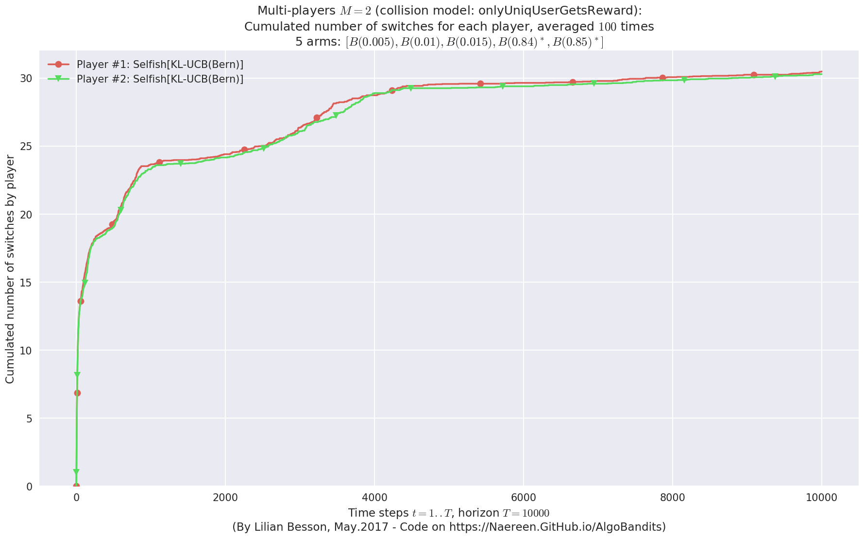
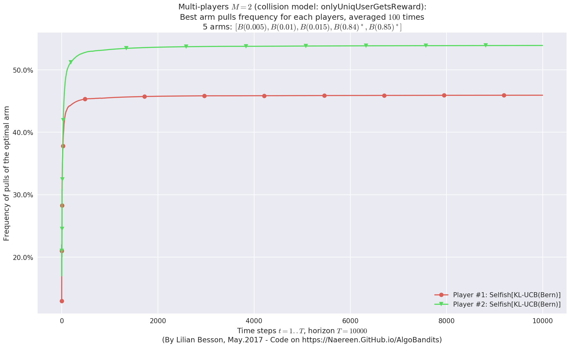
No upper bound for the non-cumulated number of collisions...
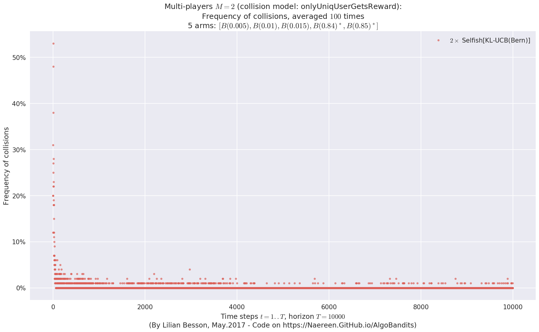
No upper bound for the non-cumulated number of collisions...

  - For #$0$: $B(0.005)$ ($0.0%$$\%$),  frequency of collisions is 3.8e-05  ...
  - For #$1$: $B(0.01)$ ($0.0%$$\%$),   frequency of collisions is 3.3e-05  ...
  - For #$2$: $B(0.015)$ ($0.0%$$\%$),  frequency of collisions is 3.4e-05  ...
  - For #$3$: $B(0.84)$ ($0.1%$$\%$),   frequency of collisions is 0.00057  ...
  - For #$4$: $B(0.85)$ ($0.1%$$\%$),   frequency of collisions is 0.000632  ...
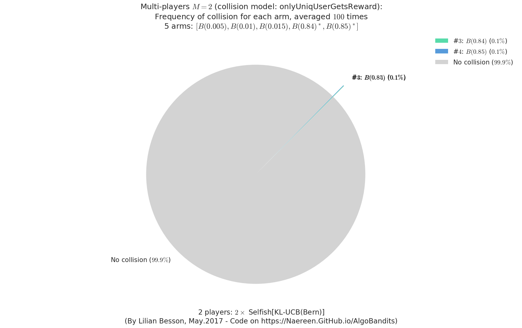
Comparing their performances
In [28]:
def plotCombined(e0, eothers, envId):
    # Centralized regret
    e0.plotRegretCentralized(envId, evaluators=eothers)
    # Fairness
    e0.plotFairness(envId, fairness="STD", evaluators=eothers)
    # Number of switches
    e0.plotNbSwitchsCentralized(envId, cumulated=True, evaluators=eothers)
    # Number of collisions - not for Centralized* policies
    e0.plotNbCollisions(envId, cumulated=True, evaluators=eothers)
In [29]:
 N = len(configuration["environment"])
for envId, env in enumerate(configuration["environment"]):
    e0, eothers = evaluators[envId][0], evaluators[envId][1:]
    plotCombined(e0, eothers, envId)
 -  For 2 players, Anandtharam et al. centralized lower-bound gave = 9 ...
 -  For 2 players, our lower bound gave = 18 ...
 -  For 2 players, the initial lower bound in Theorem 6 from [Anandkumar et al., 2010] gave = 12.1 ...

This MAB problem has:
 - a [Lai & Robbins] complexity constant C(mu) = 9.46 for 1-player problem ...
 - a Optimal Arm Identification factor H_OI(mu) = 60.00% ...
 - [Anandtharam et al] centralized lowerbound = 18,
 - Our decentralized lowerbound = 12.1,
 - [Anandkumar et al] decentralized lowerbound = 9
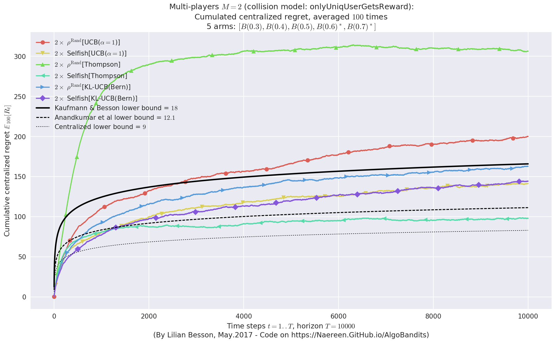
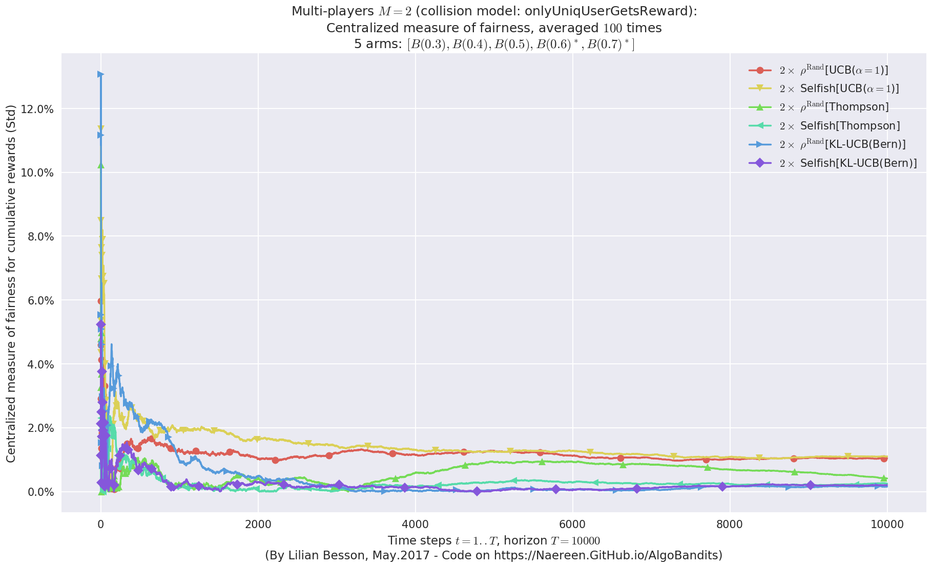
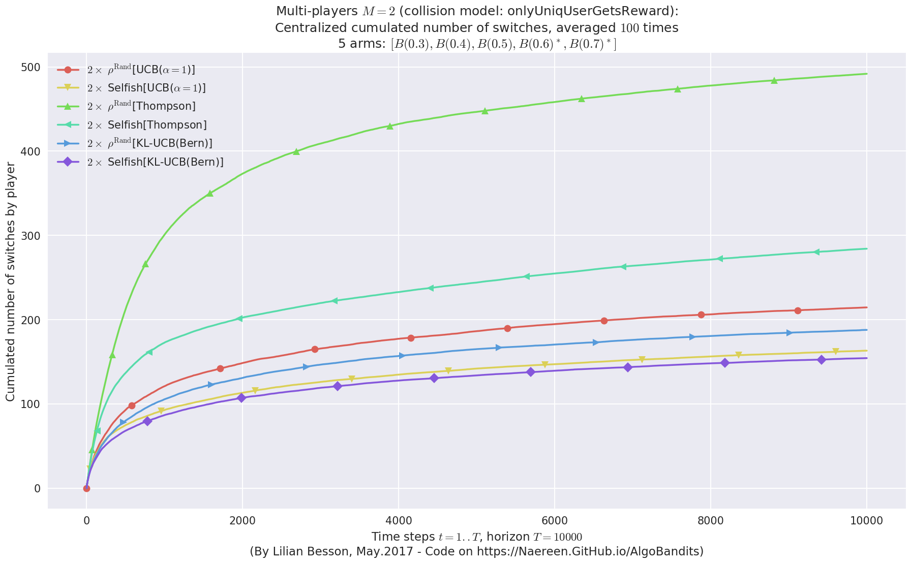
No upper bound for the non-cumulated number of collisions...
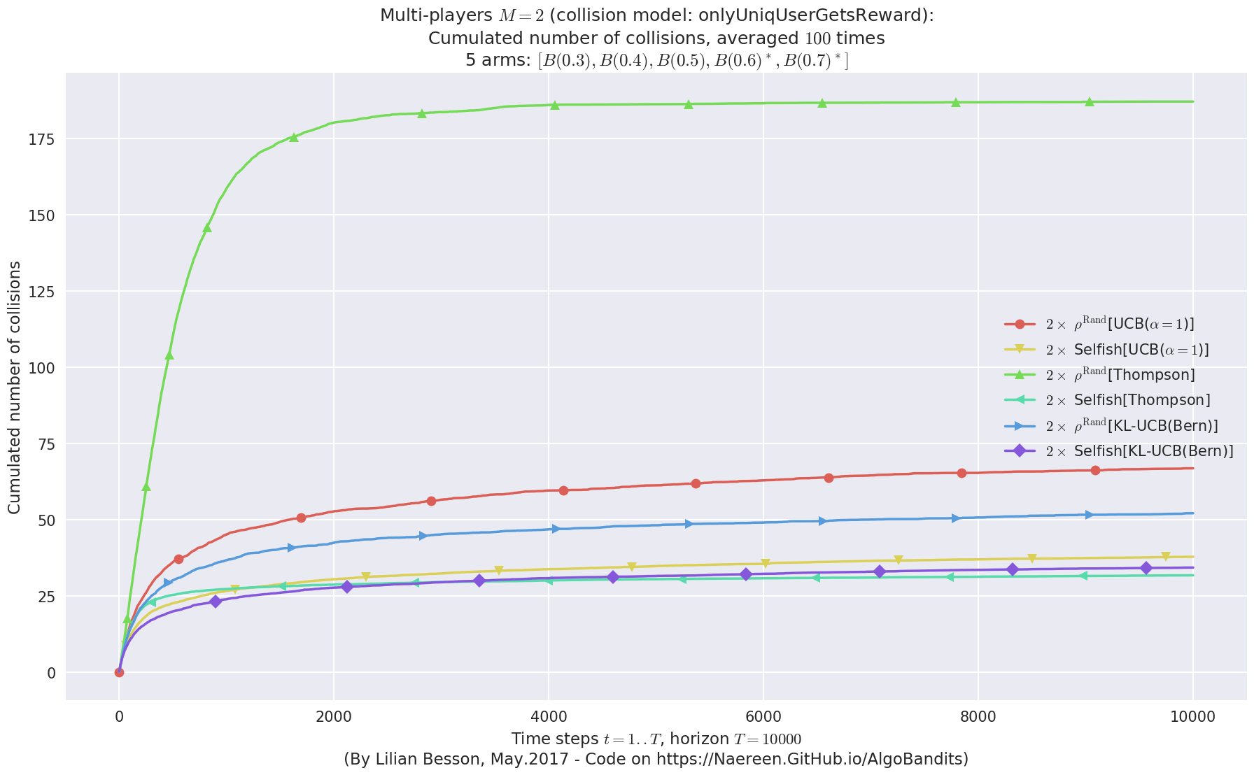
 -  For 2 players, Anandtharam et al. centralized lower-bound gave = 4.23 ...
 -  For 2 players, our lower bound gave = 8.46 ...
 -  For 2 players, the initial lower bound in Theorem 6 from [Anandkumar et al., 2010] gave = 5.35 ...

This MAB problem has:
 - a [Lai & Robbins] complexity constant C(mu) = 3.12 for 1-player problem ...
 - a Optimal Arm Identification factor H_OI(mu) = 40.00% ...
 - [Anandtharam et al] centralized lowerbound = 8.46,
 - Our decentralized lowerbound = 5.35,
 - [Anandkumar et al] decentralized lowerbound = 4.23
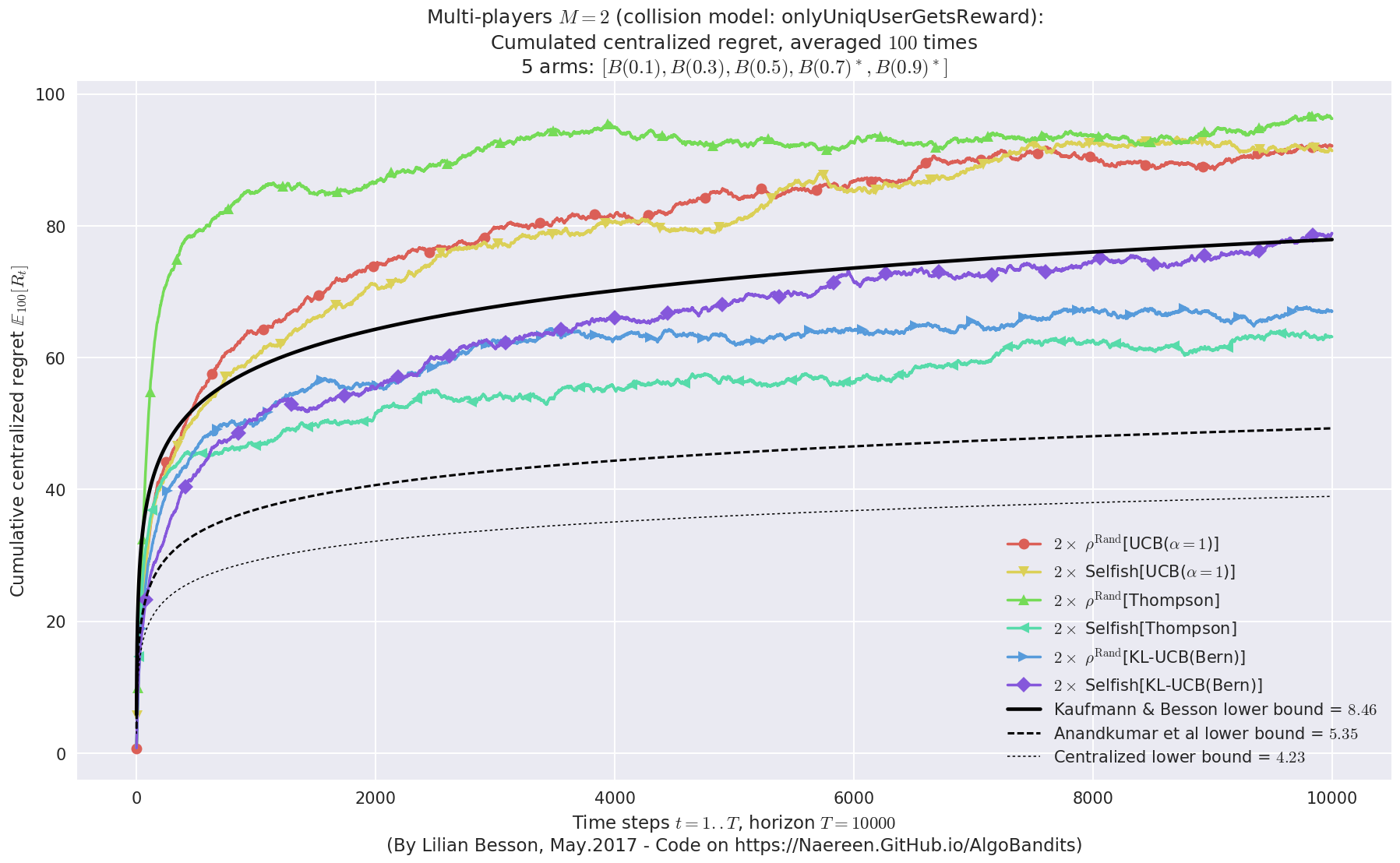
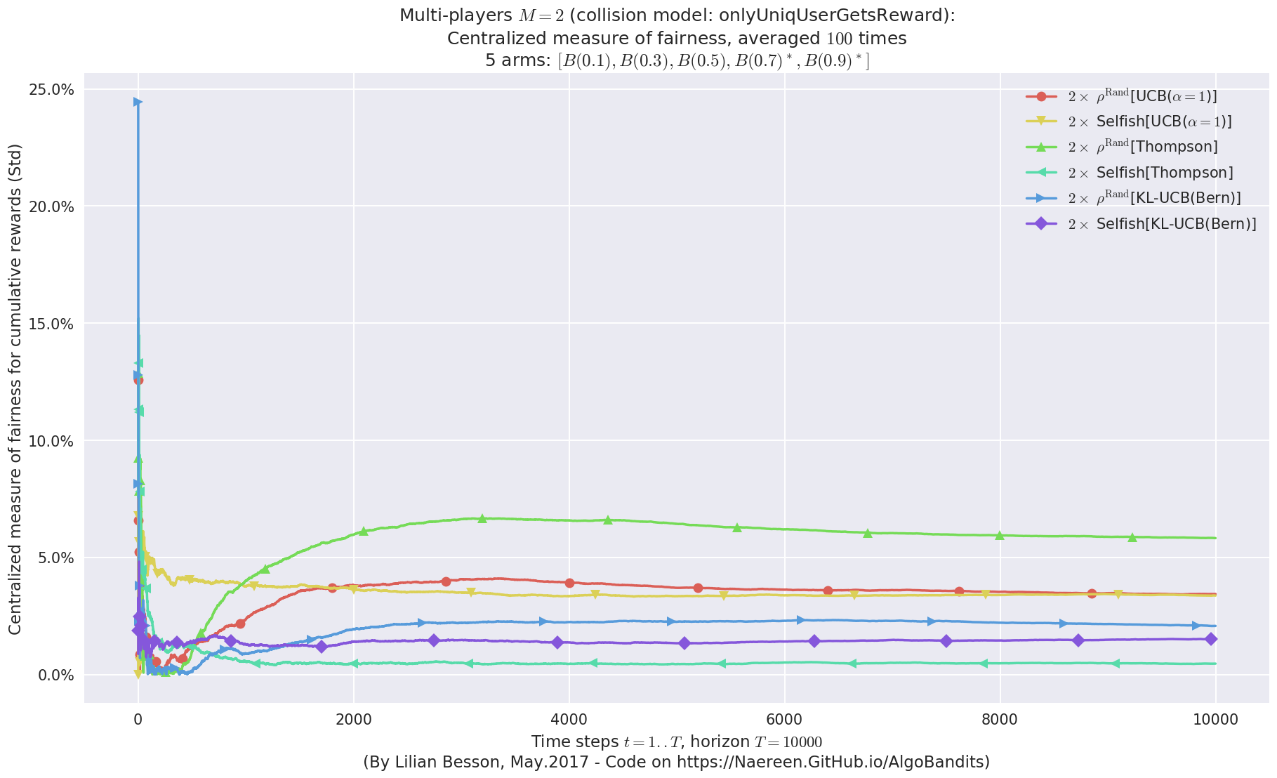
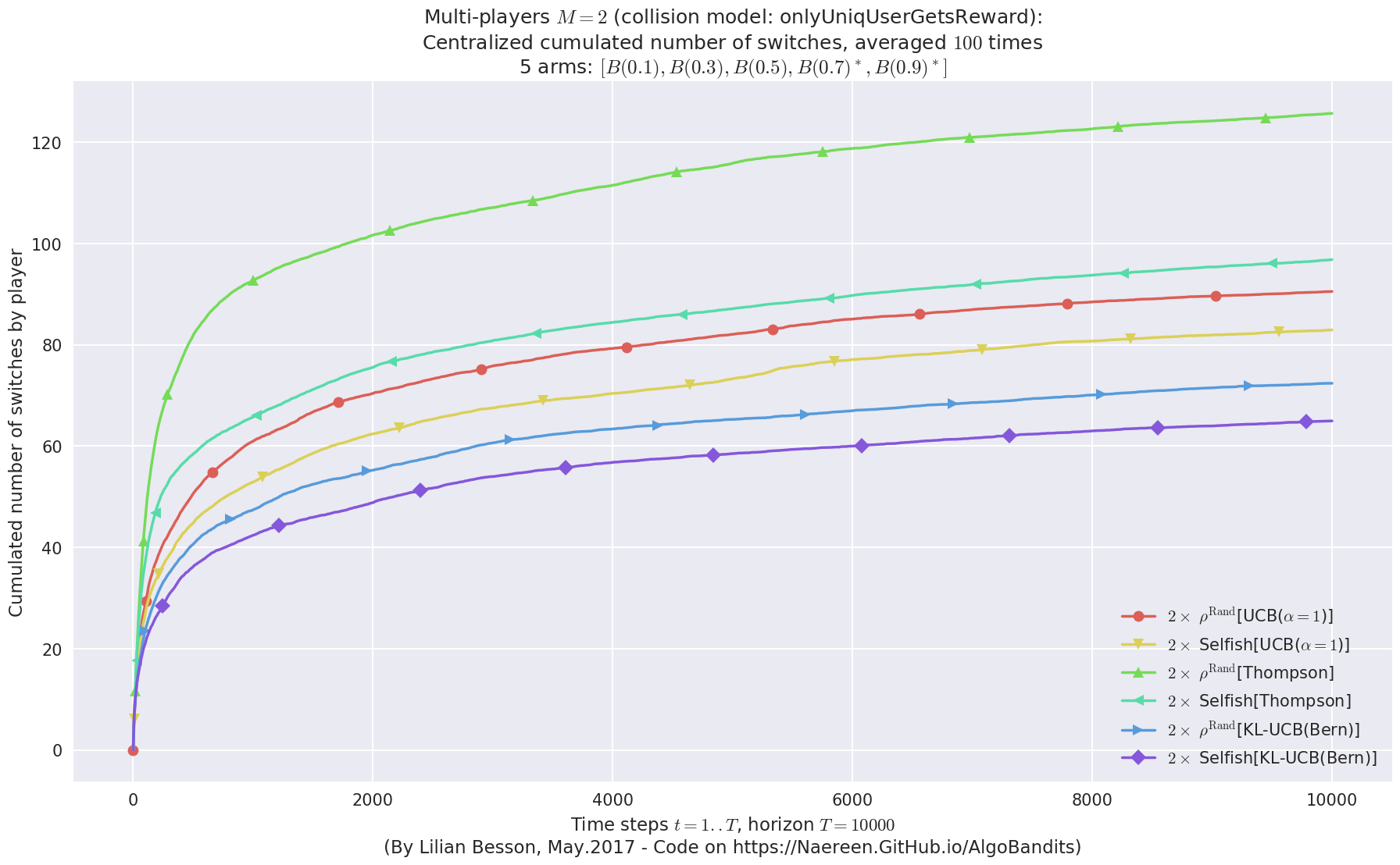
No upper bound for the non-cumulated number of collisions...
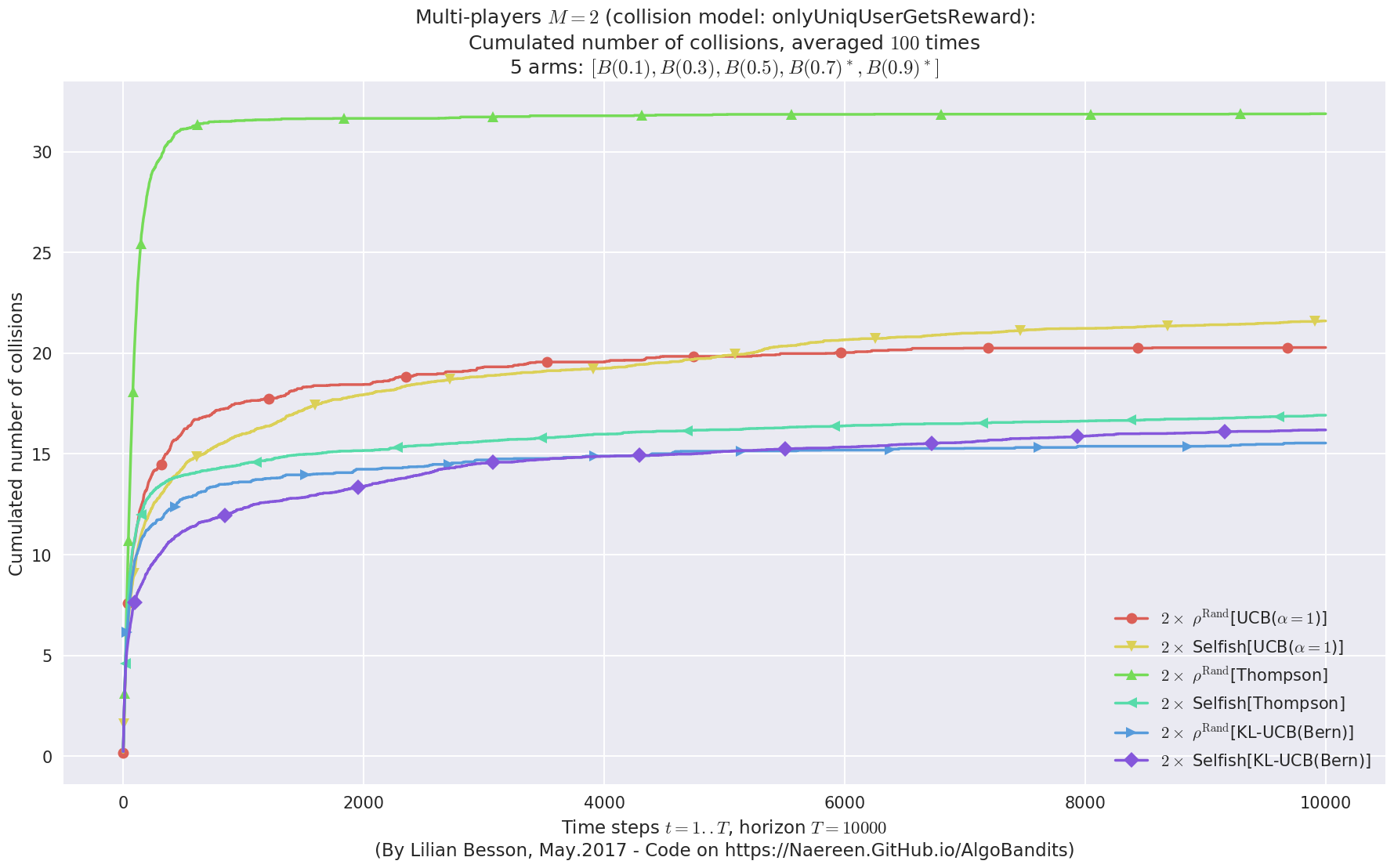
 -  For 2 players, Anandtharam et al. centralized lower-bound gave = 1.41 ...
 -  For 2 players, our lower bound gave = 2.83 ...
 -  For 2 players, the initial lower bound in Theorem 6 from [Anandkumar et al., 2010] gave = 2.78 ...

This MAB problem has:
 - a [Lai & Robbins] complexity constant C(mu) = 27.3 for 1-player problem ...
 - a Optimal Arm Identification factor H_OI(mu) = 29.40% ...
 - [Anandtharam et al] centralized lowerbound = 2.83,
 - Our decentralized lowerbound = 2.78,
 - [Anandkumar et al] decentralized lowerbound = 1.41
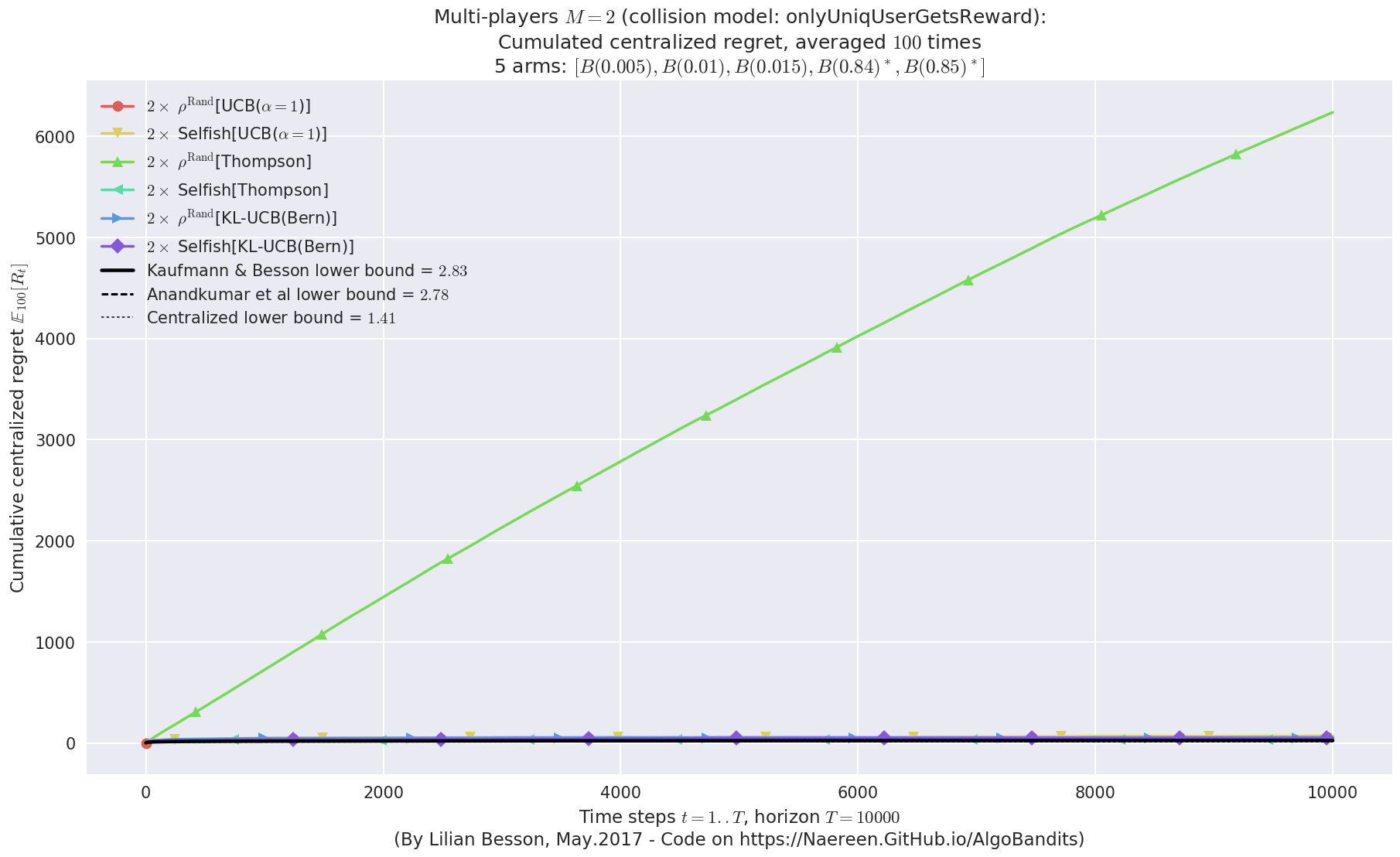
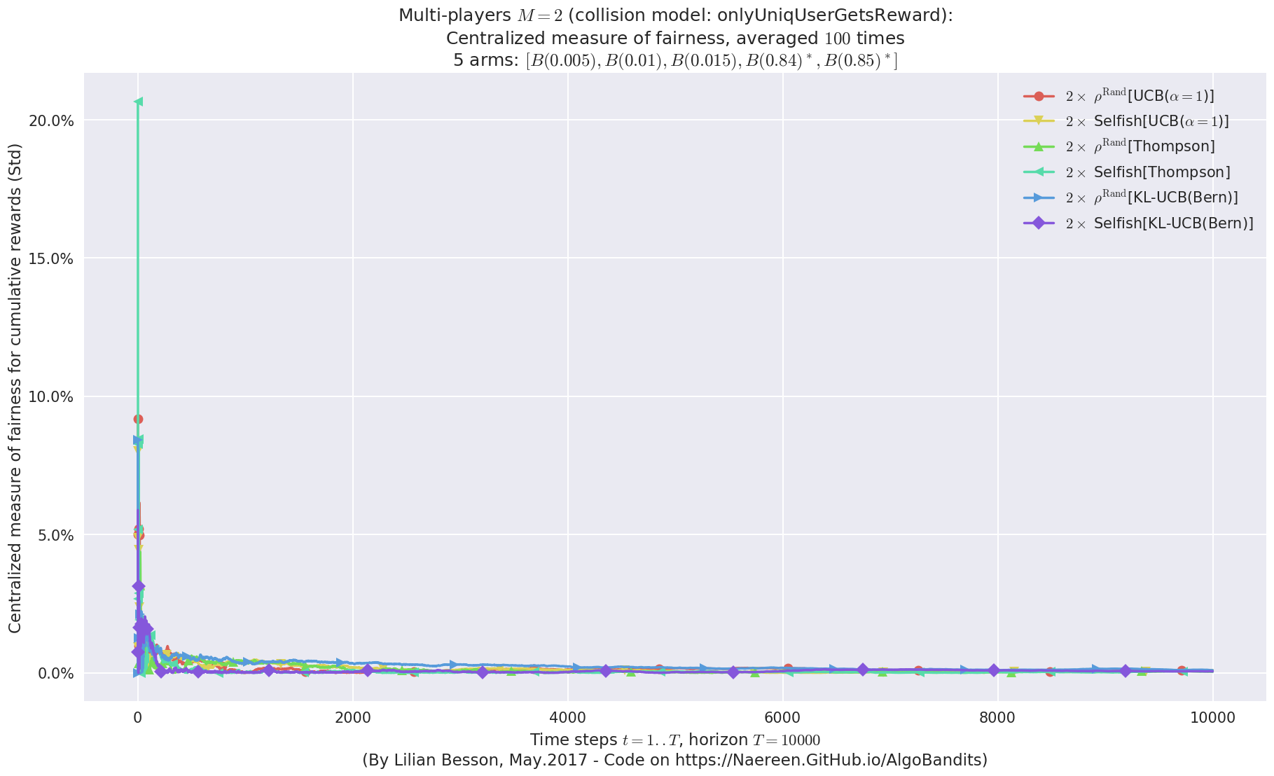

No upper bound for the non-cumulated number of collisions...
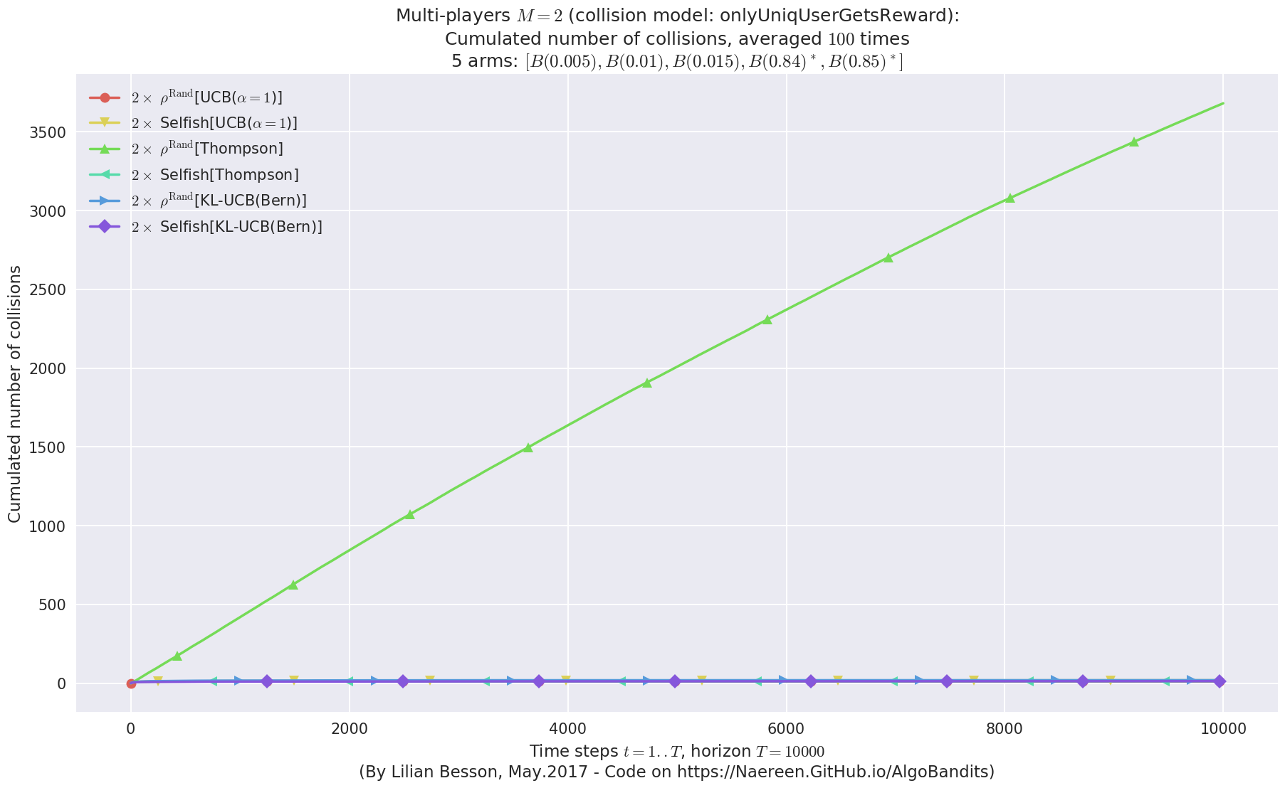
That’s it for this demo!