![]()
![]() 3D models of Random Composite Materials
3D models of Random Composite Materials
Vincent Riboulet
May-August 1999
CENTER FOR STRUCTURAL AND
APPLIED MECHANICS
|
|
|
|
Contents
Abstract……………………………………………………………………………… 3
The Work place……………………………………………………………………… 4
The University of Virginia
The Center for structures and applied
mechanics
Professor Graham’s team
Problem presentation………………….………………….………………………… 6
Material samples
Objectives
The Moving Window GMC……………………………..…………………………… 10
Overview
Application
Results
Statistical description of the data
Finite element models, stress distribution in Random
Composite………….…… 15
2D model
Relation between sxx and Elastic Modulus
Effects of the mesh
sizes
Effects of the Window
size
3D models of layered Carbon-Carbon
Composite………………………... 21
4 point Bending Test of a Beam..…………………………………… 23
Slot pull test on a
part of a jet brake disk…………….…………….
28
Conclusions…………………………………………………………………………… 33
Acknowledgements…………………………………………………………………… 34
References…………………………………………………………………………… 35
Appendix……………………………………………………………………………… 36
Photographs
4 6 6 7 7 12 12 21 22 23 28
1. University of
Virginia (the Rotunda)………………………………………..……..
4
2. Silicon carbide
fibers in titanium matrix..…………………………………………. 6
3. Graphite fiber
tow in epoxy matrix …………………………………………….….
6
4. Cellular
aluminum…………………………………………………………….…… 7
5. Functionally
graded material……………………………………………………….
7
6. Micrograph of a
functionally graded composite…………………………………... 12
7. Micrograph of a
graphite epoxy fiber tow………………………………………….
12
8. Global view of
the disk…………………………………………………………….. 21
9. Broken
lug…………………………………………………………………………. 22
10. Micrograph of
actual Carbon-Carbon composite………………………………….. 23
11. Slot Pull
test………………………………………………………………………...
28
Figures
9 11 14 17 19 23 & 25 24 26
1. Beam with varying
Young’s modulus……………………………………..………..…
8
2. Principles of the
research………………………………………………….………….. 9
3. Moving Window
GMC…………………………………………….………………... 11
4. 2D
problem………………………….…………………………….……….………....
14
5. Effects of the
Mesh size……………………………………………………………... 17
6. Effects of the
Window size………………………………………………………….. 19
7. Layered
carbon-carbon composite in configuration 1………………………….
8. 4 points bending
test………………………………………………………………… 24
9. Layered
carbon-carbon composite in configuration 2………………………………. 26
Abstract
Most models of the behavior
of composite materials assume an effective homogenized set of material
properties. These models fail to capture the true behavior of the wide variety
of composite materials that exhibit significant inherent randomness: soil,
cellular materials, concrete, particulate composites, fiber-reinforced
composites. This research project is aimed at modeling the local stress in such
materials.
My personal contribution is
the creation of 3D finite element models using Abaqus to highlight the
differences in the calculated stress values between results based on
homogenized material properties and a model where each element has individual
values for the material properties. These values have been calculated from a
sample with the Moving Window GMC technique and are put in the Abaqus code
using Fortran programs.
The specific models
presented here are a layered carbon-carbon beam under 4 point bending load and
a part of a carbon-carbon brake disk under slot-pull testing. These models are
based on real samples provided by a leading materials manufacturer in the
United States.
The training
Adviser at the
University of Virginia: Lori L. Graham
Adviser at the ENS de
Cachan: Olivier Allix
Training from the 3rd
of May to the 12th of August
The Work Place
The University, the laboratory, the team.
The University of Virginia
The University of Virginia
(which includes approximately 2000 faculty and a total full time student
enrollment of about 17000) offers professional degrees under the schools of
Architecture, Law, Medicine, Commerce, Business Administration, Education,
Engineering and Applied science. The school of engineering and applied sciences
is an integral part of the university community, which provides opportunities
for interdisciplinary work in pursuit of the basic goals of education,
research, and public service.

Photo1. University of Virginia: the Rotunda
The center for structural and solid mechanics
The
center for structural and solid mechanics is a laboratory of the Civil
Engineering Department. The computational room is well equipped with several
new PC’s and some SUN and SGI work-stations. They provide via the network
access to any computer of the engineering school, such as flemming, which was
used for most of this project.
This project is funded by the National Science Foundation, in collaboration between the Civil Engineering Department of the University of Virginia and the Mechanical Engineering Department of the University of South Carolina.
Professor Graham’s Team
Professor
Lori Graham is a full time assistant professor at the civil engineering
department of the University of Virginia. Her research focuses on
stochastic finite elements, an area that merges finite element techniques with
the principles of probabilistic mechanics to provide such information as system
reliability. Her other research interests include random heterogeneous
materials, structural dynamics, and the simulation of non-Gaussian stochastic
processes
For this project her team is composed of:
·
Aimee LeBlanc (Master )
·
Bligh Wollner (Master )
·
Eman Siragy ( Ph D )
·
Fernando Ferrante ( Master )
·
Jacob Agran (Undergraduate )
·
Kevin Smith (Undergraduate)
She also works in
collaboration with Professor Sarah Baxter of the Department of Mechanical
Engineering at the University of South Carolina
Problem presentation
Creating a model for composites
Material Samples

Many composite models assume that
inclusions such as fibers are spaced at "regular" intervals. In some
cases this assumption is valid; the image below shows a micrograph of Silicon
Carbide fibers in a titanium matrix (from “Mechanics of Composite Materials”,
by C. T. Herakovich, 1999)
Photo 2 Silicon Carbide fibers in a titanium matrix
But
this is not always true. The following are images of a few samples taken from
various composite materials. All of them present significant variation in the
position of the fibers.
·
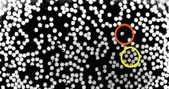
Graphite fiber tow in epoxy matrix (Kunze & Herakovich)
Photo 3 Graphite
fiber tow in epoxy matrix
The white areas correspond to graphite fibers and the dark areas
to epoxy matrix. This image of a fiber tow shows areas with relatively few
fibers (see orange-circled area on figure above), as well as clusters of many
fibers (see yellow-circled area on figure above).
·
Cellular Aluminum (Wadley)
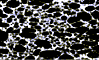
Photo 4 Cellular
Aluminum
The white areas in this image
correspond to aluminum and the black areas to voids. The void spaces vary
greatly in size, concentration, and shape.
·
Functionally Graded Material
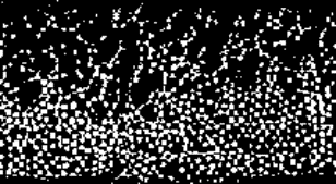
Photo 5: functionally
graded material
In this case, material properties
change not only due to functional gradation, but also because of a fairly high
degree of randomness in the fiber distribution.
We have seen that a lot of composites don’t have a regular
arrangement in their composition. It’s now interesting to have a look at the
differences in the results we get from a model assuming an homogenized material
properties and a model taking into account the variation in the material
properties. We consider a classical beam under flexion with a varying Young’s
Modulus, E(x)
E varies randomly over length (E(x))

Fig 1: Beam with
varying Yong modulus
If
we call the variation in displacement vector U, we have:
KU=P
Past research has shown small
that scale fluctuations in E(x) do
not greatly affect K and therefore U. But now if we consider
stress:
s(x)=D(x)BU
We see that s(x) is
directly impacted by fluctuations in D(x) (and therefore E(x)).
Moreover, stress is often more
important to design than displacement. So, we need appropriate descriptions of material properties for proper
analysis of stress variability.
Objectives of this work:
We are working on composites that
exhibit significant randomness in the microstructure. As we have seen, this can
have a serious impact on critical behavior such as local stresses.
In order to calculate these local
stresses, we will calculate elastic and inelastic material property fields for
a given 2-Dimensional microstructure with the moving-window GMC technique. Then
we will use these fields as input to finite element analysis (Abaqus).
Ultimately, the goal is to calculate variability of critical response of a
given structure. As we see in the graph underneath, there are 5 steps to the
research described here:
1. Collection of digitized material
micrographs
2. Generation of local material
property fields from micrographs collected in part 1, using moving-window GMC
3. Finite Element Analysis to obtain
local stress field of a given structure/ loading condition using local
properties obtained in part 2
4. Statistical characterization of
material property fields calculated in part 2 and subsequent Monte Carlo
simulation of "new" local property fields.
5. Incorporation of simulated property
fields (part 4) into finite element analysis (part 3) in order to obtain
statistics of local stresses.
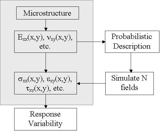
Fig
2 principles of the research.
Moving Window GMC
A micromechanical analysis: Generalized Method of
Cells.
Overview
·
The method of cells:
The method of cells (Adoubi, 1991), and
it’s extension, the generalized method of cells (Paley and Adoubi, 1995), are
approximate analytical methods for predicting the elastic as well as inelastic
response of fibrous composites. The methods can be used for two-dimensional or
three-dimensional analysis.
The theory is not the subject here. You
can find it in [1], [2] (see references). The input data are the properties of
the individual components and the geometry of the material. The overall
behavior of composites generated by the method of cells is displayed in term
of:
Effective elastic moduli
Effective coefficients of thermal
expansion
Effective thermal conductivities
Effective stress-strain response in the
inelastic region
·
The generalized method of cells
In the generalized formulation, a
repeating unit cell is subdivided into an arbitrary number of subcells. This
generalization extends the modeling capability of the method of cells to
include the following:
Modeling of variable fiber shapes
Analysis of different fiber arrays
Modeling of porosities and damage
Modeling of interfacial regions aroound
inclusios, including interfacial degradation
·
The moving window GMC
In this technique, one applies a GMC
model to a part of the sample (called the window) to calculate the local
material properties for the point in the middle of this window. The properties
of the next point are calculated by moving the window.
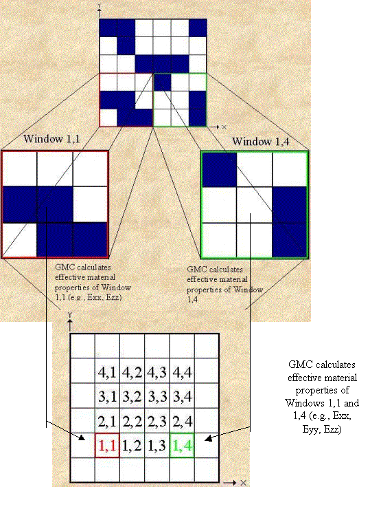
Fig 3: Moving window GMC
Application of the moving GMC
We will now look at the results that
the moving-window GMC provides for 2 different composites. We will have a more
in-depth look at the results in the finite elements 2D part.
·
Functionally Graded Microstructure
![]()
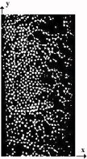
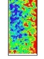
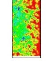
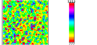
Blue and purple correspond to high
values of the moduli, red and orange are low values. Note that fiber volume
fraction increases with x coordinate. All results are based on a square window
of 7.1% x 1.8%
·

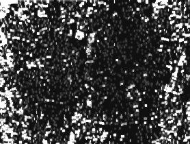
Graphite-epoxy
fiber tow


Photo 7: Micrograph of a graphite epoxy
fiber tow Local Tranverse
Elastic Modulus
Results from Moving-Window GMC
As we have seen, the moving window GMC
offers an interesting representation of the local material properties.
Currently there is work underway to identify techniques of choosing appropriate
window size: Cross-validation, Relation to underlying correlation distance,
Effect on Stress Response. Another important step is to simulate new material
property fields, based on a statistical description of the original local
material properties
Generating a Statistical Description of Data
Based on the material property fields
generated, Monte Carlo Simulations can be performed that will provide new
fields with the same statistics as the original field. In order to perform such
simulations, two important pieces of information must be estimated:
·
The
Probability Density Function defining the distribution of values at any given
point
·
The
correlation function defining the correlation between two points at various
distances apart
For more information on this part, look
at the website: http://scooter.ce.virginia.edu/~jandk/home
Such Monte Carlo simulations will be
used as input to finite element analyses, providing statistics on the maximum
stress for a number of samples of the same material.
Finite
element analysis
Stress Distribution in Random Composite
2D Finite Element
Analysis
This work is a part of the Ph.D. of
Eman Siragy, which has not been published yet. I would like to thank her and
Professor Graham for allowing me to use it. The goal here is to have an idea of
the size of the mesh and the size of the windows in the moving window GMC in
order to get accurate results. The problem is a 2D square under uniform
traction. The material is a composite with random placed circular fibers.

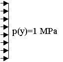
Fig 4 : 2D problem
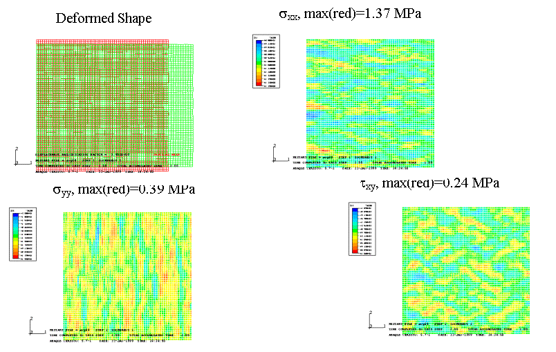
Transverse Elastic Modulus Ezz
sxx, max=1.37 MPa
Relation between sxx
and Elastic Modulus
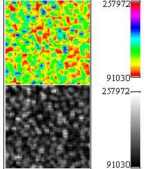
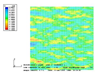
We see here that there is only
approximately 60% correlation between Exx and sxx. This shows us that the configuration is as important as
the local elastic modulus in calculating local stresses.
1.
Effects of the mesh sizes
·
sxx for
various mesh sizes
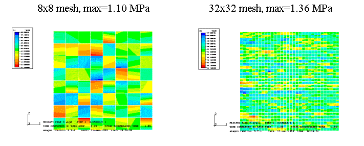
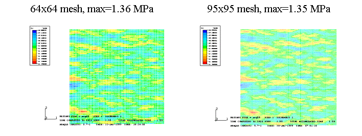
The mesh size has strong impact if the
mesh is too coarse.
·
Maximum
and Minimum Stress vs Mesh for 5%x5% Window Size
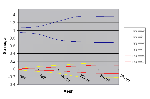
Fig5: Effects of the mesh size.
We see that the results for stress
converge between 32x32 mesh and 64x64 mesh.
We will now try to change the window
size of underlying material property fields in order to know the effects of the
Window size.
2. Effects of the
Window size
·
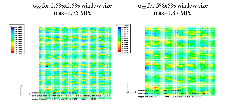
sxx for 2.5%x2.5% window size and 5%x5%
window size
There is a difference of over 20% in
results after changing the window size in the moving-window GMC analysis. We
can conclude that window size has a large impact on local stress results
·
“Exact”
Results for sxx
To get rid of the effects of the mesh,
we now use a 200x200 mesh as a basis of comparison for the result with
different window and mesh size. The stress pattern is similar to those of other
meshes
With this mesh, we have:
Maximum stress in fiber elements= 3.59
MPa; Maximum stress in matrix elements=1.90 MPa
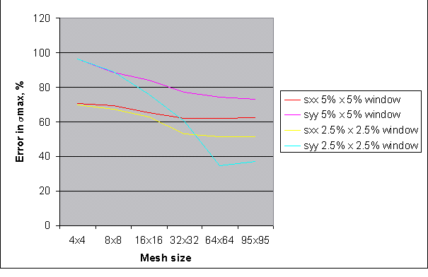
Fig 5: Effects of the window size
To compare the effects of the size of the window, we have to compare the yellow and red line (Sxx ) and the purple and blue (Syy ). We see that the results are equal for the very coarse mesh and that they begin to differ when the mesh becomes finer. The difference, especially for Syy becomes important.
·
Ratio
of local stress sxx to local yield stress sYxx
In this
example, Matrix is assumed to have a yield stress of 300.5 Mpa and Fiber
assumed to have an infinite yield stress
Transverse
Yield Stress sYxx:
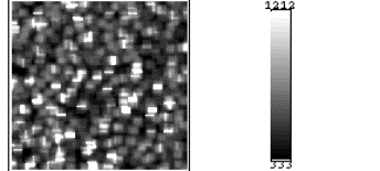
We see that areas of high elastic
moduli tend to have higher corresponding local yield stresses.
Let’s Calculate the maximum ratio of local stress sxx to local yield stress sYxx , for the 64x64 element mesh, when pressure load
p=100 MPa:
5%x5% window: 36.7% of
yield
2.5%x2.5% window: 42.2% of
yield
200x200 mesh: 63.0%
of yield
Difference has decreased somewhat from 62% to 41% (for the 5%x5%
windowing) and 51% to 33% (for the 2.5%x2.5% windowing). These results are
interesting, as they suggest that consideration of stress alone may not be
appropriate without accounting for some local maximum stress, such as yield
stress. Clearly, this idea merits further study
Conclusions on the 2D models
•In
calculating local stresses, configuration is as important as local elastic
moduli or local fiber volume fraction
•For
a given field of material properties, the finite element results converged with
increasing mesh - smaller windowing scheme called for finer meshing to achieve
convergence
•Consideration
of local stress variation relative to a consistent benchmark (e.g., yield
stress from the same GMC windows) yields better results, may be more rational
•Nature
of sample (fibers placed at purely random locations) leads to short correlation
distance of underlying material - worst-case scenario?
Technique may be applied to
real materials, in 2D
3D Examples
The goal is now to apply the technique we have applied on the 2D square
to real 3D samples. A carbon-carbon jet brake disk supplied by one of the
leading materials manufacturer in the United States, which is working with the
team, is used for this analysis.
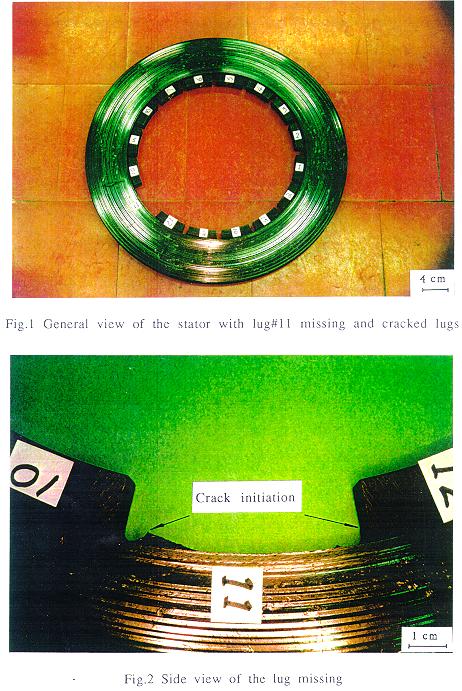
Photo 8 : Global view of the disk
As we can see there is a problem with
fracture at the lug.
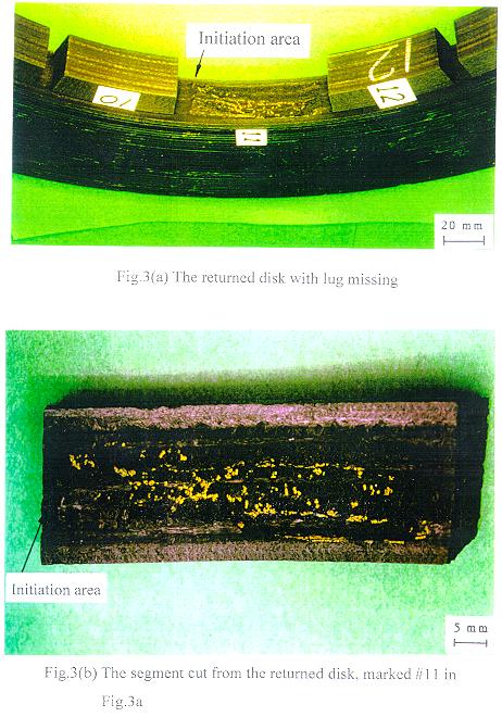
Photo 9 : broken lug
Our goal is to apply our technique to see the effect on the local stress
at the base of the lug, in order to learn if the difference in local stress can
explain the rupture.
The manufacturer of the disk gave us information on 2 tests they had
performed. The first one is a test of a 4-layer beam of this material, and the
second one is a slot pull test on a part of the disk.
Layered
Carbon-Carbon Composite
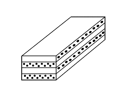
Fig 7: layered composite in
configuration 1

The beam is made of 4 layers of carbon
carbon composite wich are in 0 90 direction. 2 models will be made, depending
on the direction of the bottom fibers.
To begin we used this model of the fibers:
![]()
Micrograph
Assumed in first Finite Element Models
Then we used data from a real sample. The values given here are the one
we got with the real material. Values of the first model are available in the
appendix.
![]()
Photo 10 :
Micrograph of actual Carbon-Carbon Composite - 1 layer
The Material is assumed not to vary in fiber direction
Loading: 4-point
Bending Test
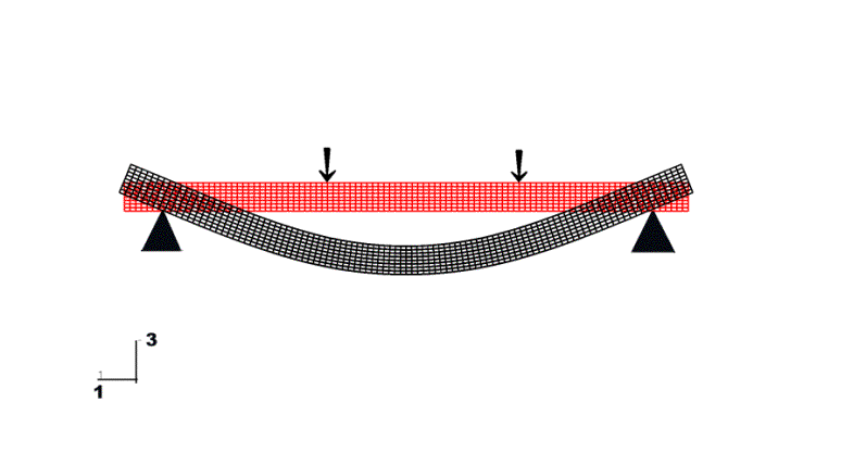
Fig 8 : 4
points bending test
This test was made in order to
get an idea of the flexural strength. It was performed per ASTM D970. The
specimen is 0.25 inches thick, 0.80 inches wide, and 5.0 inches in length. The
outer span (support) is 4.2 inches while the inner span (load point ) is 1.4
inches. They found a typical structural strength of 15.0 Ksi.
We compare 2
models. One assumed that the composite is homogeneous. Each element has the
average values of the material properties. The second model takes the values of
the moving window GMC. To do that, a Fortran program reads the values and then
makes all the calculation to give to each element is own values. The output is
a text file which is used as input for abaqus.
The materials
properties given by the Moving GMC are given for a rectangle of 1layer * 0.80.
There are 1800 * 140 points For each different mesh an average value is
calculated on the values of the point inside an element to give to this element
is value. The elements that are next in the fiber direction get the same value.
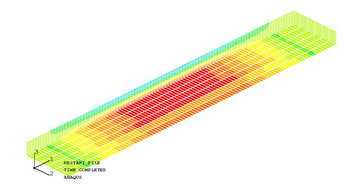
Beam with bottom
fibers in direction y
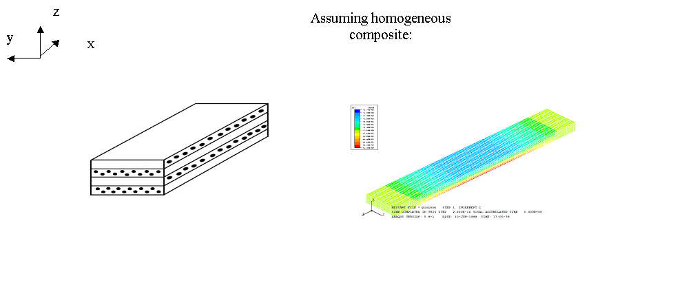
Fig 7 : Layered composite in
configuration 1
Using varying microstructure as input:
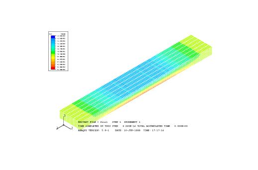 Fibers in bottom layer follow y-direction
The values of sxx are:
·
Homogeneous materials:
sxxmax=137 MPa
sxxmin=-177 MPa
·
Varying microstructure:
sxxmax=156 MPa
sxxmin=-191 MPa
Beam with bottom fibers in direction x
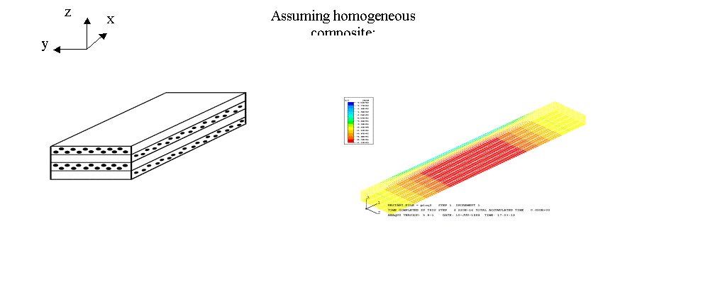
Fig 9 : Layered composite in
configuration 2
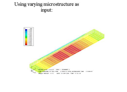
Fibers in bottom layer
follow
y-direction
The values of sxx are:
·
Homogeneous materials:
sxxmax=112 MPa
sxxmin=-201 Mpa
·
Varying microstructure:
sxxmax=130 MPa
sxxmin=-201 MPa
The results show an interesting difference in the
values of sxx. So we decided to make more
models of the beam in order to make some comparisons with different meshes as
we have done in 2D. The beam has 4 layers in the thickness so at least 4
elements in the direction of the thickness. We have to keep some proportions
for the shape of the elements, the computational time of the first model was
pretty low (about 30minutes). So we decide to make models with more fine
meshes. 6 models were created:
·
100*6*8=4800 elements
·
125*20*12=30000
·
150*24*16=57600
·
175*28*16=78400
·
200*32*20=128000
·
225*36*28=226800
All this models have been created
together with a special enumeration to allow the use of a unique fortran
program, which takes in account all the possibilities. You can find all the
(big) listing of theses models in the appendix.
The problem I encountered is that
the computer ran out of memory. I was using Flemming.seas.virginia.edu, an IBM
RS6000 with 1 Go of RAM. With the help of a system engineer, we logged the
Abaqus job and discovered that it was trying to write a file which was bigger
than 1Go, which is the default limit size of a file under the Unix system. So
we set the limit to 2 Go, which is the maximum allocated by the OS, but then we
encounter a lack of disk space in my account. We finally decided to switch to
the IBM SP, which is a big multiprocessor RS600 (24 processors in parallel )
and which is used for big and long running jobs. As I was the first in the lab
to use it, I went through some troubles to configure everything in my Unix
account. I finally succeeded but to discover that the SP suffers the same
limitations as Flemming in the maximum size of a file, so my jobs didn’t
worked. You can find the HTML 4 tutorial I have written on the use of the SP in
the appendix.
Theses computational problems were
very frustrating as I spent a lot of time on my models (especially the huge
unique fortran program). It really shows the limitations of the numerical
problems in 3D. Hopefully, one will be able to use my work when a system
engineer will have fixed all the problems.
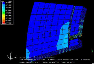
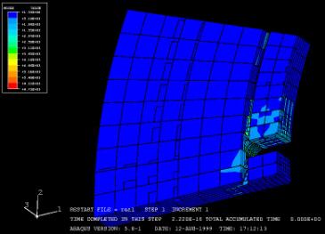
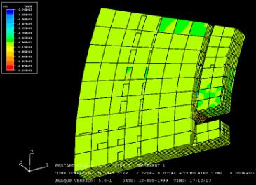
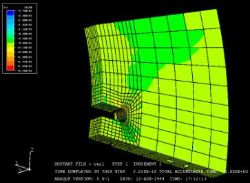
Slot-pull specimen
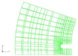

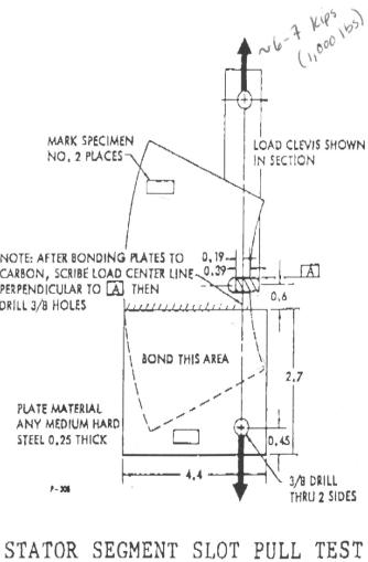
This test
was made in order to know the resistance of the slot. The disk is cut in the
radial direction so that there is only one slot remaining. Then there is a load
on this slot of about 6 Kips (1000 lbs).


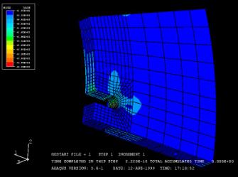
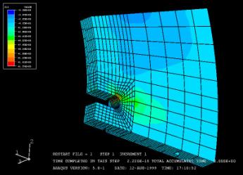
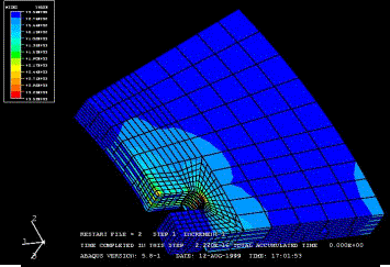
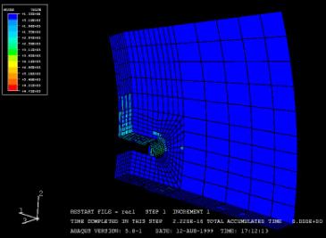
![]() The geometry of
the disk is really complicated and was difficult to model under abaqus without
the help of a pre processor (which automatically creates the mesh). Basically,
two meshes were created, one for the inside of the disk and the other one for
the friction part. Then I “tied” the
corresponding nodes of the 2 models. The other problem is that I used
cylindrical coordinates for the disk but that the fixation, were the disk is
bond is not radial.
The geometry of
the disk is really complicated and was difficult to model under abaqus without
the help of a pre processor (which automatically creates the mesh). Basically,
two meshes were created, one for the inside of the disk and the other one for
the friction part. Then I “tied” the
corresponding nodes of the 2 models. The other problem is that I used
cylindrical coordinates for the disk but that the fixation, were the disk is
bond is not radial.
This
time, I also made 2 models for the homogenized values but as the differences
were not important, I made one model with a varying microstructure.
Disk with bottom fibers in radial direction
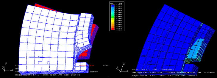
|
|
srr |
sqq |
szz |
Mises |
|
Min |
-5.28E2 |
-3.83E3 |
-9.44E1 |
1.63 |
|
Max |
1.57E03 |
3.83E03 |
3.57E2 |
4.29E3 |
|
|
srr |
sqq |
szz |
Mises |
|
Min |
-2.39E3 |
-2.86E3 |
-3.07E2 |
3.59 |
|
Max |
1.88E3 |
3.6E3 |
3.27E3 |
3.52E3 |
|
|
srr |
sqq |
szz |
Mises |
|
Min |
-2.67E3 |
-7.11E3 |
-9.53E2 |
1.32 |
|
Max |
2.24E3 |
7.73E3 |
9.9E2 |
6.73E3 |
|
|
|
srr |
sqq |
szz |
Mises |
|
Homogeneous dir R |
Min |
-5.28E2 |
-3.83E3 |
-9.44E1 |
1.63 |
|
Max |
1.57E03 |
3.83E03 |
3.57E2 |
4.29E3 |
|
|
Homogeneous dir q |
Min |
-2.39E3 |
-2.86E3 |
-3.07E2 |
3.59 |
|
Max |
1.88E3 |
3.6E3 |
3.27E3 |
3.52E3 |
|
|
Varying
microstructure |
Min |
-2.67E3 |
-7.11E3 |
-9.53E2 |
1.32 |
|
Max |
2.24E3 |
7.73E3 |
9.9E2 |
6.73E3 |
We see
here that the results with the varying microstructure are not so different from
the one we get assuming a homogeneous composite. This can be related to the
fact that the mesh of the model is pretty coarse, so the material value for
each element of the model is an average of a lot of points, minimizing the
variation of the values.
Conclusions
The application of the moving-Window GMC technique to model
the behavior of composite materials (layered carbon-carbon composite with
randomly placed circular fibers) proved to be a very interesting technique.
The extended study of a 2D square under tension load showed
us that:
-window size has a large impact on local stress results.
-the results are equal for very coarse meshes and that they
begin to differ when the mesh becomes finer.
-consideration of stress alone may not be appropriate
without accounting for some local maximum stress, such as yield stress. (this
idea merits further study)
The beam and slot pull test were the first 3D models
generated using this technique. What took the most time was generating the mesh
"by hand". A preprocessor could have been much faster but would not
have give us the same control other the enumeration, which proved to be very
helpful while writing the Fortran programs (alloting to each element its
material properties). I tried to make an exhaustive study in 3D as it has been
made in 2D, but faced a lot of numeric problems ( memory limitations ). A major
future direction of research is to try to overcome theses problems in order to
get an idea of the importance of window and mesh size.
Acknowledgments
I
would like to thank the following persons:
In France
Olivier
Allix, my adviser at the ENS de Cachan for this training, to have accepted to
be my adviser and to have followed me.
Sebastien
Le-Loch, who has put me in contact with the UVA team and has given me a lot of
wise advises.
In the USA
All
the staff of the international center, to have given to me a friendly place to
stay.
Cindy
Sites, secretary of the department, for her help in all the administrative
approach, and to have loan to me a so useful bike for the summer.
Jim
Damberg, to have allowed me to use all his tools, and for is help.
Brad
Sayler, computer system engineers, for his help in setting up a working
station.
E
H. Carruth and Jeffrey L. Chisholm , ITC staff, system engineer on the Abaqus
station, for all their help to try to fix all the computer related problems.
Carlt
T. Herakovich, emeritus professor, to have allowed me to contact Professor
Graham, and for his discussions in French!
Furman
W. Barton, Civil engineering department, for his help with the Abaqus license
and all the Abaqus documentation
Eman
Siragy, Ph.D. Candidate, for all her precious advises with Abaqus.
And most of all
Lori
L. Graham, supervisor of the training, to let me free and to trust me for the
choices of my research ways, for her welcome and all she made for me before and
during this 3 months.
References
[1] C.T. Herakovich,
Mechanics of Fibrous
Composites, 1997
[2] M.Paley and J.Aboudi
Micromechanical analysis of
composites by the generalized method of cell model,
Mechanic of Materials, 1992
[3]All the Abaqus
documentation, especially the example manual.
[4]Installation guide for
Linux, all the ITC on-line documentation about Unix.


