### IEEE WCNC: **« Aggregation of Multi-Armed Bandits Learning Algorithms for Opportunistic Spectrum Access »**
- *Date* :date: : $16$th of April $2018$
- *Who:* [Lilian Besson](https://GitHub.com/Naereen/slides/) :wave: , PhD Student in France, co-advised by
| *Christophe Moy*
@ CentraleSupélec
& IETR, Rennes | *Émilie Kaufmann*
@ Inria, Lille |
|:---:|:---:|
|   |  |
> See our paper [`HAL.Inria.fr/hal-01705292`](https://hal.inria.fr/hal-01705292)
---
# Introduction
- Cognitive Radio (CR) is known for being one of
the possible solution to tackle the spectrum scarcity issue
- Opportunistic Spectrum Access (OSA) is a good model
for CR problems in **licensed bands**
- Online learning strategies, mainly using multi-armed bandits (MAB) algorithms, were recently proved to be efficient `[Jouini 2010]`
- :boom: But there are many different MAB algorithms…
which one should you choose in practice?
$\Longrightarrow$ we propose to use an online learning algorithm to also decide
which algorithm to use, to be more robust and adaptive to unknown environments.
---
# :timer_clock: Outline
1. Opportunistic Spectrum Access
2. Multi-Armed Bandits
3. MAB algorithms
4. Aggregation of MAB algorithms
5. Illustration
### Please :pray:
Ask questions *at the end* if you want!
---
# 1. Opportunistic Spectrum Access
- Spectrum scarcity is a well-known problem
- Different range of solutions…
- Cognitive Radio is one of them
- Opportunistic Spectrum Access is a kind of cognitive radio
---
# Communication & interaction model
 - :phone: Primary users are occupying $K$ radio channels
- :iphone: Secondary users can sense and exploit free channels:
want to **explore** the channels, and learn to **exploit** the best one
- Discrete time for everything $t\geq1,t\in\mathbb{N}$
---
# 2. Multi-Armed Bandits
## Model
- Again $K \geq 2$ resources (*e.g.*, channels), called **arms**
- Each time slot $t=1,\ldots,T$, you must choose one arm, denoted $A(t)\in\{1,\ldots,K\}$
- You receive some reward $r(t) \sim \nu_k$ when playing $k = A(t)$
- **Goal:** maximize your sum reward $\sum\limits_{t=1}^{T} r(t)$, or expected $\sum\limits_{t=1}^{T} \mathbb{E}[r(t)]$
- Hypothesis: rewards are stochastic, of mean $\mu_k$. *E.g.*, Bernoulli
## Why is it famous?
Simple but good model for **exploration/exploitation** dilemma.
---
# 3. MAB algorithms
- Main idea: index $I_k(t)$ to approximate the quality of each arm $k$
- First example: *UCB algorithm*
- Second example: *Thompson Sampling*
---
# 3.1 Multi-Armed Bandit algorithms
### Often *index* based
- Keep *index* $I_k(t) \in \mathbb{R}$ for each arm $k=1,\ldots,K$
- Always play $A(t) = \arg\max I_k(t)$
- $I_k(t)$ should represent our belief of the *quality* of arm $k$ at time $t$
### Example: "Follow the Leader"
- $X_k(t) := \sum\limits_{s < t} r(s) \bold{1}(A(s)=k)$ sum reward from arm $k$
- $N_k(t) := \sum\limits_{s < t} \bold{1}(A(s)=k)$ number of samples of arm $k$
- And use $I_k(t) = \hat{\mu}_k(t) := \frac{X_k(t)}{N_k(t)}$.
---
# 3.2 First example of algorithm (2002)
*Upper Confidence Bounds* algorithm (UCB)
- Instead of using $I_k(t) = \frac{X_k(t)}{N_k(t)}$, add an exploration term
$$ I_k(t) = \frac{X_k(t)}{N_k(t)} + \sqrt{\frac{\alpha \log(t)}{2 N_k(t)}} $$
### Parameter $\alpha$: tradeoff exploration *vs* exploitation
- Small $\alpha$: focus more on **exploitation**
- Large $\alpha$: focus more on **exploration**
### :boom: Problem: how to choose "the good $\alpha$" for a certain problem?
---
# 3.3 Second example of algorithm (1933)
*Thompson sampling* (TS)
- Choose an initial belief on $\mu_k$ (uniform) and a prior $p^t$ (*e.g.*, a Beta prior on $[0,1]$)
- At each time, update the prior $p^{t+1}$ from $p^t$ using Bayes theorem
- And use $I_k(t) \sim p^t$ as *random* index
### Example with Beta prior, for binary rewards
- $p^t = \mathrm{Beta}(1 + \text{nb successes}, 1 + \text{nb failures})$.
- Mean of $p^t$ $= \frac{1 + X_k(t)}{2 + N_k(t)} \simeq \hat{\mu}_k(t)$.
### :boom: How to choose "the good prior" for a certain problem?
---
# 4. Aggregation of MAB algorithms
## Problem
- How to choose which algorithm to use?
- But also… Why commit to one only algorithm?
## Solutions
- Offline benchmarks?
- Or online selections from a pool of algorithms?
## $\hookrightarrow$ Aggregation?
> Not a new idea, studied from the 90s in the ML community.
- Also use online learning to *select the best algorithm*!
---
## 4.1 Basic idea for online aggregation
If you have $\mathcal{A}_1,\ldots,\mathcal{A}_N$ different algorithms
- At time $t=0$, start with a uniform distribution $\pi^0$ on $\{1,\ldots,N\}$
(to represent the **trust** in each algorithm)
- At time $t$, choose $a^t \sim \pi^t$, then play with $\mathcal{A}_{a^t}$
- Compute next distribution $\pi^{t+1}$ from $\pi^t$:
+ increase $\pi^{t+1}_{a^t}$ if choosing $\mathcal{A}_{a^t}$ gave a good reward
+ or decrease it otherwise
## Problems
1. How to increase $\pi^{t+1}_{a^t}$ ?
2. What information should we give to which algorithms?
---
## 4.2 Overview of the *Exp4* aggregation algorithm (2002)
> For rewards in $r(t) \in [-1,1]$.
- Use $\pi^t$ to choose randomly the algorithm to trust, $a^t \sim \pi^t$
- Play its decision, $A_{\text{aggr}}(t) = A_{a^t}(t)$, receive reward $r(t)$
- And give feedback of observed reward $r(t)$ only to this one
- Increase or decrease $\pi^t_{a^t}$ using an exponential weight:
$$ \pi^{t+1}_{a^t} := \pi^{t}_{a^t} \times \exp\left(\eta_t \times \frac{r(t)}{\pi^t_{a^t}}\right).$$
- Renormalize $\pi^{t+1}$ to keep a distribution on $\{1,\ldots,N\}$
- Use a sequence of decreasing *learning rate* $\eta_t = \frac{\log(N)}{t \times K}$
(cooling scheme, $\eta_t \to 0$ for $t\to\infty$)
---
## Use an *unbiased* estimate of the rewards
Using directly $r(t)$ to update trust probability yields a biased estimator
- So we use instead $\hat{r}(t) = r(t) / \pi^t_{a}$ if we trusted algorithm $\mathcal{A}_a$
- This way
$$\mathbb{E}[\hat{r}(t)] = \sum\limits_{a=1}^N \mathbb{P}(a^t = a) \mathbb{E}[r(t) / \pi^t_{a}]$$
$$= \mathbb{E}[r(t)] \sum\limits_{a=1}^N \frac{\mathbb{P}(a^t = a)}{\pi^t_{a}} = \mathbb{E}[r(t)]
$$
---
## 4.3 Our *Aggregator* aggregation algorithm
Improves on *Exp4* by the following ideas:
- First let each algorithm vote for its decision $A_1^t,\ldots,A_N^t$
- Choose arm $A_{\text{aggr}}(t) \sim p_j^{t+1} := \sum\limits_{a=1}^N \pi_a^t \mathbf{1}(A_a^t = j)$
- Update trust for each of the trusted algorithm, not only one
(*i.e.*, if $A_a^t = A_{\text{aggr}}^t$)
$\hookrightarrow$ faster convergence
- Give feedback of reward $r(t)$ to *each* algorithm!
(and not only the one trusted at time $t$)
$\hookrightarrow$ each algorithm have more data to learn from
---
# 5. Some illustrations
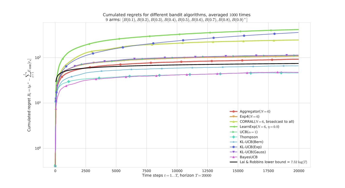
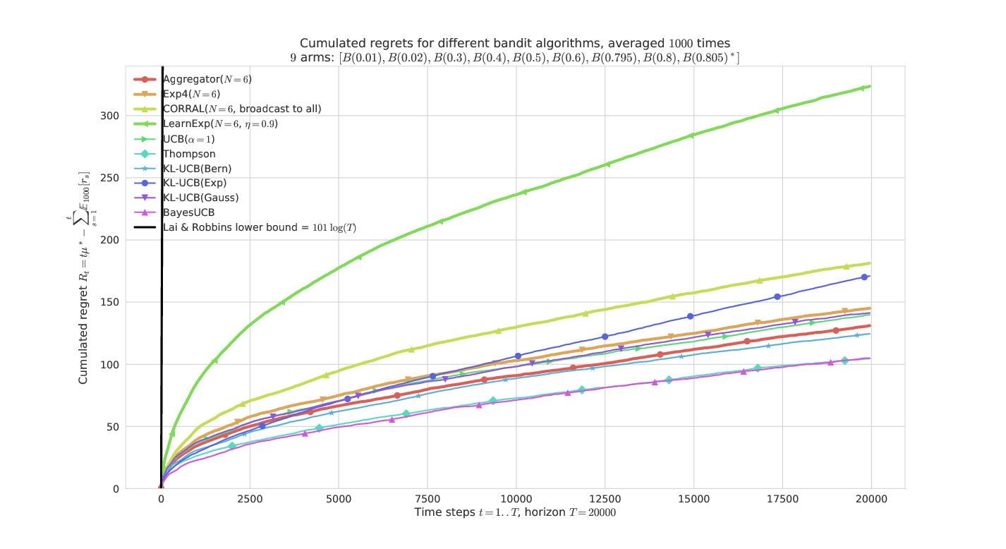
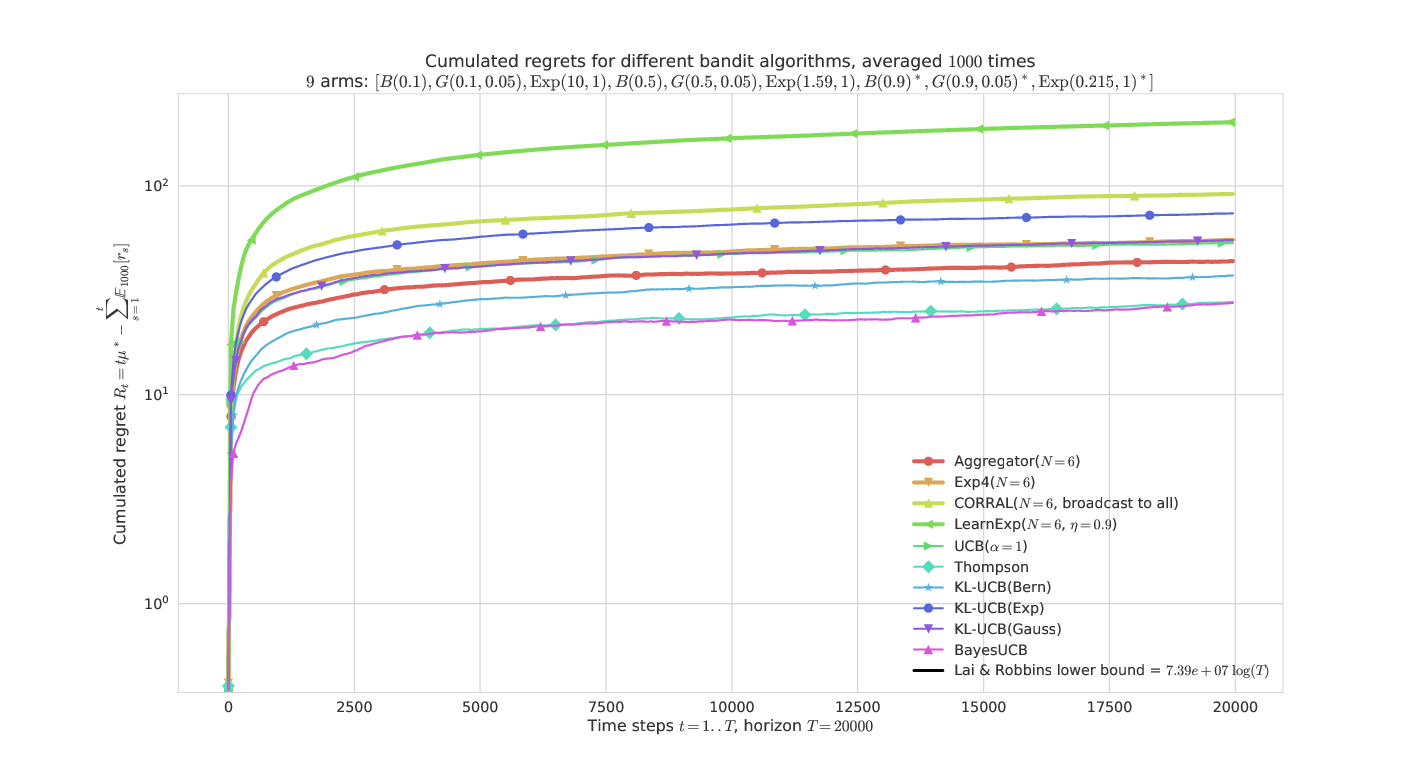
- Artificial simulations of stochastic bandit problems
- Bernoulli bandits but not only (also Gaussian, Exponential)
- Pool of different algorithms (UCB, Thompson Sampling etc)
- Compared with other state-of-the-art algorithms for *expert aggregation* (Exp4, CORRAL, LearnExp)
- What is plotted it the *regret* for problem of means $\mu_1,\ldots,\mu_K$ :
$$ R_T^{\mu}(\mathcal{A}) = \max_k (T \mu_k) - \sum_{t=1}^T \mathbb{E}[r(t)] $$
- Regret is known to be lower-bounded by $C(\mu) \log(T)$
and upper-bounded by $C'(\mu) \log(T)$ for efficient algorithms
---
# On a simple Bernoulli problem
---
# On a "hard" Bernoulli problem
---
# On a mixed problem
---
# Conclusion (1/2)
- Online learning can be a powerful tool for Cognitive Radio, and many other real-world applications
- Many formulations exist, a simple one is the Multi-Armed Bandit
- Many algorithms exist, to tackle different situations
- It's hard to know before hand which algorithm is efficient for a certain problem…
- Online learning can also be used to select *on the run*
which algorithm to prefer, for a specific situation!
---
# Conclusion (2/2)
- Our algorithm **Aggregator** is **efficient and easy to implement**
- For $N$ algorithms $\mathcal{A}_1,\ldots,\mathcal{A}_N$, it costs $\mathcal{O}(N)$ memory,
and $\mathcal{O}(N)$ extra computation time at each time step
- For stochastic bandit problem, it outperforms empirically
the other state-of-the-arts (Exp4, CORRAL, LearnExp).
### See our paper: [`HAL.Inria.fr/hal-01705292`](https://hal.inria.fr/hal-01705292)
### See our code for experimenting with bandit algorithms
Python library, open source at [`SMPyBandits.GitHub.io`](https://SMPyBandits.GitHub.io)
Thanks for listening !
 - :phone: Primary users are occupying $K$ radio channels
- :iphone: Secondary users can sense and exploit free channels:
want to **explore** the channels, and learn to **exploit** the best one
- Discrete time for everything $t\geq1,t\in\mathbb{N}$
---
# 2. Multi-Armed Bandits
## Model
- Again $K \geq 2$ resources (*e.g.*, channels), called **arms**
- Each time slot $t=1,\ldots,T$, you must choose one arm, denoted $A(t)\in\{1,\ldots,K\}$
- You receive some reward $r(t) \sim \nu_k$ when playing $k = A(t)$
- **Goal:** maximize your sum reward $\sum\limits_{t=1}^{T} r(t)$, or expected $\sum\limits_{t=1}^{T} \mathbb{E}[r(t)]$
- Hypothesis: rewards are stochastic, of mean $\mu_k$. *E.g.*, Bernoulli
## Why is it famous?
Simple but good model for **exploration/exploitation** dilemma.
---
# 3. MAB algorithms
- Main idea: index $I_k(t)$ to approximate the quality of each arm $k$
- First example: *UCB algorithm*
- Second example: *Thompson Sampling*
---
# 3.1 Multi-Armed Bandit algorithms
### Often *index* based
- Keep *index* $I_k(t) \in \mathbb{R}$ for each arm $k=1,\ldots,K$
- Always play $A(t) = \arg\max I_k(t)$
- $I_k(t)$ should represent our belief of the *quality* of arm $k$ at time $t$
### Example: "Follow the Leader"
- $X_k(t) := \sum\limits_{s < t} r(s) \bold{1}(A(s)=k)$ sum reward from arm $k$
- $N_k(t) := \sum\limits_{s < t} \bold{1}(A(s)=k)$ number of samples of arm $k$
- And use $I_k(t) = \hat{\mu}_k(t) := \frac{X_k(t)}{N_k(t)}$.
---
# 3.2 First example of algorithm (2002)