Table of Contents

1  Trying to use Unsupervised Learning algorithms for a Gaussian bandit problem

1.1  Creating the Gaussian bandit problem

1.2  Getting data from a first phase of uniform exploration

1.3  Fitting an Unsupervised Learning algorithm

1.4  Using the prediction to decide the next arm to sample

1.5  Manual implementation of basic Gaussian kernel fitting

1.6  Implementing a Policy from that idea

1.6.1  Basic algorithm

1.6.2  A variant, by aggregating samples

1.6.3  Implementation

1.7  Comparing its performance on this Gaussian problem

1.7.1  Configuring an experiment

1.7.2  Running an experiment

1.7.3  Visualizing the results

1.8  Another experiment, with just more Gaussian arms

1.8.1  Running the experiment

1.8.2  Visualizing the results

1.8.3  Very good performance!

1.9  Another experiment, with Bernoulli arms

1.9.1  Running the experiment

1.9.2  Visualizing the results

1.10  Conclusion

1.10.1  Non-logarithmic regret

1.10.2  Comparing time complexity

1.10.3  Not so efficient for Bernoulli arms

---

Trying to use Unsupervised Learning algorithms for a Gaussian bandit problem

This small Jupyter notebook presents an experiment, in the context of Multi-Armed Bandit problems (MAB).

I am trying to answer a simple question:

“Can we use generic unsupervised learning algorithm, like Kernel Density estimation or Ridge Regression, instead of MAB algorithms like UCB or Thompson Sampling ?

I will use my SMPyBandits library, for which a complete documentation is available, here at https://smpybandits.github.io/, and the scikit-learn package.

Creating the Gaussian bandit problem

First, be sure to be in the main folder, and import the `MAB class <https://smpybandits.github.io/docs/Environment.MAB.html#Environment.MAB.MAB>`__ from the ``Environment` package <https://smpybandits.github.io/docs/Environment.html#module-Environment>`__:

import numpy as np

from sys import path
path.insert(0, '..')

from Environment import MAB

 - Setting dpi of all figures to 110 ...
 - Setting 'figsize' of all figures to (19.8, 10.8) ...
Info: Using the Jupyter notebook version of the tqdm() decorator, tqdm_notebook() ...

And also, import the `Gaussian class <https://smpybandits.github.io/docs/Arms.Gaussian.html#Arms.Gaussian.Gaussian>`__ to create Gaussian-distributed arms.

from Arms import Gaussian

Info: numba.jit seems to be available.

# Just improving the ?? in Jupyter. Thanks to https://nbviewer.jupyter.org/gist/minrk/7715212
from __future__ import print_function
from IPython.core import page
def myprint(s):
    try:
        print(s['text/plain'])
    except (KeyError, TypeError):
        print(s)
page.page = myprint

Gaussian?

Init signature: Gaussian(mu, sigma=0.05, mini=0, maxi=1)
Docstring:
Gaussian distributed arm, possibly truncated.

- Default is to truncate into [0, 1] (so Gaussian.draw() is in [0, 1]).
Init docstring: New arm.
File:           ~/ownCloud/cloud.openmailbox.org/Thèse_2016-17/src/SMPyBandits.git/Arms/Gaussian.py
Type:           type

Let create a simple bandit problem, with 3 arms, and visualize an histogram showing the repartition of rewards.

means = [0.45, 0.5, 0.55]
M = MAB(Gaussian(mu, sigma=0.2) for mu in means)

Creating a new MAB problem ...
  Taking arms of this MAB problem from a list of arms 'configuration' = <generator object <genexpr> at 0x7f8363cc4888> ...
 - with 'arms' = [G(0.45, 0.2), G(0.5, 0.2), G(0.55, 0.2)]
 - with 'means' = [ 0.45  0.5   0.55]
 - with 'nbArms' = 3
 - with 'maxArm' = 0.55
 - with 'minArm' = 0.45

This MAB problem has:
 - a [Lai & Robbins] complexity constant C(mu) = 12 ...
 - a Optimal Arm Identification factor H_OI(mu) = 61.67% ...
 - with 'arms' represented as: $[G(0.45, 0.2), G(0.5, 0.2), G(0.55, 0.2)^*]$

M.plotHistogram(horizon=1000000)

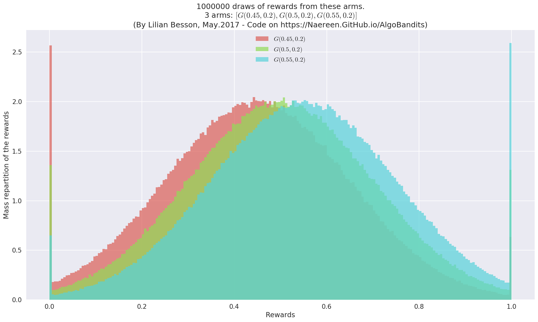
As we can see, the rewards of the different arms are close. It won’t be easy to distinguish them.

Then we can generate some draws, from all arms, from time \(t=1\) to \(t=T_0\), for let say \(T_0 = 1000\) :

T_0 = 1000
shape = (T_0,)
draws = np.array([ b.draw_nparray(shape) for b in M.arms ])

draws

array([[ 0.24726137,  0.61569462,  0.59461208, ...,  0.39197396,
         0.45834681,  0.30944561],
       [ 0.52334399,  0.65358504,  0.43245798, ...,  0.74248213,
         0.7482495 ,  0.49452348],
       [ 0.66065217,  0.60462104,  0.64908096, ...,  0.78747225,
         0.47917156,  0.39706533]])

The empirical means of each arm can be estimated, quite easily, and could be used to make all the decisions from \(t \geq T_0 + 1\).

empirical_means = np.mean(draws, axis=1)

empirical_means

array([ 0.46016747,  0.50465274,  0.55415233])

Clearly, the last arm is the best. And the empirical means \(\hat{\mu}_k(t)\) for \(k=1,\dots,K\), are really close to the true one, as \(T_0 = 1000\) is quite large.

def relative_error(x, y):
    return np.abs(x - y) / x

relative_error(means, empirical_means)

array([ 0.02259438,  0.00930549,  0.00754969])

That’s less than \(3\%\) error, it’s already quite good!

Conclusion : If we have “enough” samples, and the distribution are not too close, there is no need to do any learning: just pick the arm with highest mean, from now on, and you will be good!

best_arm_estimated = np.argmax(empirical_means)
best_arm = np.argmax(means)
assert best_arm_estimated == best_arm, "Error: the best arm is wrongly estimated, even after {} samples.".format(T_0)

---

Getting data from a first phase of uniform exploration

But maybe \(T_0 = 1000\) was really too large…

Let assume that the initial data was obtained from an algorithm which starts playing by exploring every arm, uniformly at random, until it gets “enough” data.

• On the one hand, if we ask him to sample each arm \(1000\) times, of course the empirical mean \(\hat{\mu_k(t)}\) will correctly estimate the true mean \(\mu_k\) (if the gap \(\Delta = \min_{i \neq j} |\mu_i - \mu_j|\) is not too small).
• But on the other hand, starting with a long phase of uniform exploration will increase dramatically the regret.

What if we want to use the same technique on very few data? Let see with \(T_0 = 10\), if the empirical means are still as close to the true ones.

np.random.seed(10000)  # for reproducibility of the error best_arm_estimated = 1
T_0 = 10
draws = np.array([ b.draw_nparray((T_0, )) for b in M.arms ])
empirical_means = np.mean(draws, axis=1)
empirical_means

array([ 0.42070333,  0.51071708,  0.50317952])

relative_error(means, empirical_means)
best_arm_estimated = np.argmax(empirical_means)
best_arm_estimated
assert best_arm_estimated == best_arm, "Error: the best arm is wrongly estimated, even after {} samples.".format(T_0)

array([ 0.06510371,  0.02143416,  0.08512815])

1

---------------------------------------------------------------------------
AssertionError                            Traceback (most recent call last)
<ipython-input-17-15e056f5ef63> in <module>()
      2 best_arm_estimated = np.argmax(empirical_means)
      3 best_arm_estimated
----> 4 assert best_arm_estimated == best_arm, "Error: the best arm is wrongly estimated, even after {} samples.".format(T_0)

AssertionError: Error: the best arm is wrongly estimated, even after 10 samples.

Clearly, if there is not enough sample, the *empirical mean* estimator can be wrong. It will not always be wrong with so few samples, but it can.

---

Fitting an Unsupervised Learning algorithm

We should use the initial data for more than just getting empirical means.

Let use a simple Unsupervised Learning algorithm, implemented in the scikit-learn (``sklearn`) <http://scikit-learn.org/>`__ package: 1D Kernel Density estimation.

from sklearn.neighbors.kde import KernelDensity

First, we need to create a model.

Here we assume to know that the arms are Gaussian, so fitting a Gaussian kernel will probably work the best. The bandwidth parameter should be of the order of the variances \(\sigma_k\) of each arm (we used \(0.2\)).

kde = KernelDensity(kernel='gaussian', bandwidth=0.2)
kde

KernelDensity(algorithm='auto', atol=0, bandwidth=0.2, breadth_first=True,
       kernel='gaussian', leaf_size=40, metric='euclidean',
       metric_params=None, rtol=0)

Then, we will feed it the initial data, obtained from the initial phase of uniform exploration, from \(t = 1, \dots, T_0\).

draws
draws.shape

array([[ 0.19578187,  0.48522741,  0.39075672,  0.51538576,  0.25531612,
         0.4955362 ,  0.28613439,  0.47144451,  0.64505553,  0.46639478],
       [ 0.40467549,  0.20156569,  0.41930701,  0.63895565,  0.54243056,
         0.51819797,  0.19022907,  0.49103453,  0.81135267,  0.88942214],
       [ 0.39297198,  0.12215761,  0.29714829,  0.60899744,  0.71129785,
         0.60553406,  0.30123099,  0.70745487,  0.70040608,  0.584596  ]])

(3, 10)

We need to use the transpose of this array, as the data should have shape (n_samples, n_features), i.e., of shape (10, 3) here.

kde.fit?

Signature: kde.fit(X, y=None)
Docstring:
Fit the Kernel Density model on the data.

Parameters
----------
X : array_like, shape (n_samples, n_features)
    List of n_features-dimensional data points.  Each row
    corresponds to a single data point.
File:      /usr/local/lib/python3.5/dist-packages/sklearn/neighbors/kde.py
Type:      method

kde.fit(draws.T)

KernelDensity(algorithm='auto', atol=0, bandwidth=0.2, breadth_first=True,
       kernel='gaussian', leaf_size=40, metric='euclidean',
       metric_params=None, rtol=0)

The `score_samples(X) <http://scikit-learn.org/stable/modules/generated/sklearn.neighbors.KernelDensity.html#sklearn.neighbors.KernelDensity.score_samples>`__ method can be used to evaluate the density on sample data (i.e., the likelihood of each observation).

kde.score_samples(draws.T)

array([ 0.74775249,  0.38689241,  0.8415668 ,  1.15395093,  0.78990714,
        1.14875055,  0.65704831,  1.05109219,  0.69428901,  0.64198648])

For instance, based on the means \([0.45, 0.5, 0.55]\), the sample \([10, -10, 0]\) should be very unlikely, while \([0.4, 0.5, 0.6]\) will be more likely. And the vector of empirical means is a very likely observation as well.

kde.score(np.array([10, -10, 0]).reshape(1, -1))
kde.score(np.array([0.4, 0.5, 0.6]).reshape(1, -1))
kde.score(empirical_means.reshape(1, -1))

-2432.9531169042129

1.1497424000393375

1.1001537768074523

---

Using the prediction to decide the next arm to sample

Now that we have a model of Kernel Density estimation, we can use it to generate some random samples.

kde.sample?

Signature: kde.sample(n_samples=1, random_state=None)
Docstring:
Generate random samples from the model.

Currently, this is implemented only for gaussian and tophat kernels.

Parameters
----------
n_samples : int, optional
    Number of samples to generate. Defaults to 1.

random_state : RandomState or an int seed (0 by default)
    A random number generator instance.

Returns
-------
X : array_like, shape (n_samples, n_features)
    List of samples.
File:      /usr/local/lib/python3.5/dist-packages/sklearn/neighbors/kde.py
Type:      method

Basically, that means we can use this model to predict what the next output of the 3 arms (constituting the Gaussian problem) will be.

Let see this with one example.

np.random.seed(1)
one_sample = kde.sample()
one_sample

array([[ 0.38558697,  0.23762342,  0.92208452]])

one_draw = M.draw_each()
one_draw

array([ 0.48799428,  0.38957079,  0.69945781])

Of course, the next random rewards from the arms have no reason to be close to predicted ones…

But maybe we can use the prediction to choose the arm with highest sample? And hopefully this will be the best arm, at least in average!

best_arm_sampled = np.argmax(one_sample)
best_arm_sampled
assert best_arm_sampled == best_arm, "Error: the best arm is wrongly estimated from a random sample, even after {} observations.".format(T_0)

2

Manual implementation of basic Gaussian kernel fitting

We can also implement manually a simple 1D Unsupervised Learning algorithm, which fits a Gaussian kernel (i.e., a distribution \(\mathcal{N}(\mu,\sigma)\)) on the 1D data, for each arm.

Let start with a base class, showing the signature any Unsupervised Learning should have to be used in our policy (defined below).

# --- Unsupervised fitting models

class FittingModel(object):
    """ Base class for any fitting model"""

    def __init__(self, *args, **kwargs):
        """ Nothing to do here."""
        pass

    def __repr__(self):
        return str(self)

    def fit(self, data):
        """ Nothing to do here."""
        return self

    def sample(self, shape=1):
        """ Always 0., for instance."""
        return 0.

    def score_samples(self, data):
        """ Always 1., for instance."""
        return 1.

    def score(self, data):
        """ Log likelihood of the point (or the vector of data), under the current Gaussian model."""
        return np.log(np.sum(self.score_samples(data)))

And then, the SimpleGaussianKernel class, using `scipy.stats.norm.pdf <https://docs.scipy.org/doc/scipy/reference/generated/scipy.stats.norm.html>`__ to evaluate the log-probability of an observation.

import scipy.stats as st


class SimpleGaussianKernel(FittingModel):
    """ Basic Unsupervised Learning algorithm, which simply fits a 1D Gaussian on some 1D data."""

    def __init__(self, loc=0., scale=1., *args, **kwargs):
        r""" Starts with :math:`\mathcal{N}(0, 1)`, by default."""
        self.loc = float(loc)
        self.scale = float(scale)

    def __str__(self):
        return "N({:.3g}, {:.3g})".format(self.loc, self.scale)

    def fit(self, data):
        """ Use the mean and variance from the 1D vector data (of shape `n_samples` or `(n_samples, 1)`)."""
        self.loc, self.scale = np.mean(data), np.std(data)
        return self

    def sample(self, shape=1):
        """ Return one or more sample, from the current Gaussian model."""
        if shape == 1:
            return np.random.normal(self.loc, self.scale)
        else:
            return np.random.normal(self.loc, self.scale, shape)

    def score_samples(self, data):
        """ Likelihood of the point (or the vector of data), under the current Gaussian model, component-wise."""
        return st.norm.pdf(data, loc=self.loc, scale=np.sqrt(self.scale))

---

Implementing a Policy from that idea

Based on that idea, we can implement a policy, following the common API of all the policies of my framework.

Basic algorithm

• Initially : create \(K\) Unsupervised Learning algorithms \(\mathcal{U}_k(0)\), \(k\in\{1,\dots,K\}\), for instance KernelDensity estimators.

• For the first \(K \times T_0\) time steps, each arm \(k \in \{1, \dots, K\}\) is sampled exactly \(T_0\) times, to get a lot of initial observations for each arm.

• With these first \(T_0\) (e.g., \(50\)) observations, train a first version of the Unsupervised Learning algorithms \(\mathcal{U}_k(t)\), \(k\in\{1,\dots,K\}\).

• Then, for the following time steps, \(t \geq T_0 + 1\) :

  • Once in a while (every \(T_1 =\) fit_every steps, e.g., \(100\)), retrain all the Unsupervised Learning algorithms :

    • For each arm \(k\in\{1,\dots,K\}\), use all the previous observations of that arm to train the model \(\mathcal{U}_k(t)\).

  • Otherwise, use the previously trained model :

    • Get a random sample, \(s_k(t)\) from the \(K\) Unsupervised Learning algorithms \(\mathcal{U}_k(t)\), \(k\in\{1,\dots,K\}\) :

      \[\forall k\in\{1,\dots,K\}, \;\; s_k(t) \sim \mathcal{U}_k(t).\]

    • Chose the arm \(A(t)\) with highest sample :

      \[A(t) \in \arg\max_{k\in\{1,\dots,K\}} s_k(t).\]

    • Play that arm \(A(t)\), receive a reward \(r_{A(t)}(t)\) from its (unknown) distribution, and store it.

A variant, by aggregating samples

A more robust (and so more correct) variant could be to use a bunch of samples, and use their mean to give \(s_k(t)\) :

• Get a bunch of \(M\) random samples (e.g., \(50\)), \(s_k^i(t)\) from the \(K\) Unsupervised Learning algorithms \(\mathcal{U}_k(t)\), \(k\in\{1,\dots,K\}\) :

  \[\forall k\in\{1,\dots,K\}, \;\; \forall i\in\{1,\dots,M\}, \;\; s_k^i(t) \sim \mathcal{U}_k(t).\]

• Average them to get \(\hat{s_k}(t)\) :

  \[\forall k\in\{1,\dots,K\}, \;\; \hat{s_k}(t) := \frac{1}{M} \sum_{i=1}^{M} s_k^i(t).\]

• Chose the arm \(A(t)\) with highest mean sample :

  \[A(t) \in \arg\max_{k\in\{1,\dots,K\}} \hat{s_k}(t).\]

Implementation

In code, this gives the following:

class UnsupervisedLearning(object):
    """ Generic policy using an Unsupervised Learning algorithm, from scikit-learn.

    - Warning: still highly experimental!
    """

    def __init__(self, nbArms, estimator=KernelDensity,
                 T_0=10, fit_every=100, meanOf=50,
                 lower=0., amplitude=1.,  # not used, but needed for my framework
                 *args, **kwargs):
        self.nbArms = nbArms
        self.t = -1
        T_0 = int(T_0)
        self.T_0 = int(max(1, T_0))
        self.fit_every = int(fit_every)
        self.meanOf = int(meanOf)
        # Unsupervised Learning algorithm
        self._was_fitted = False
        self._estimator = estimator
        self._args = args
        self._kwargs = kwargs
        self.ests = [ self._estimator(*self._args, **self._kwargs) for _ in range(nbArms) ]
        # Store all the observations
        self.observations = [ [] for _ in range(nbArms) ]

    def __str__(self):
        return "UnsupervisedLearning({.__name__}, $T_0={:.3g}$, $T_1={:.3g}$, $M={:.3g}$)".format(self._estimator, self.T_0, self.fit_every, self.meanOf)

    def startGame(self):
        """ Reinitialize everything."""
        self.t = -1
        self.ests = [ self._estimator(*self._args, **self._kwargs) for _ in range(self.nbArms) ]

    def getReward(self, armId, reward):
        """ Store this observation."""
        # print("   - At time {}, we saw {} from arm {} ...".format(self.t, reward, armId))  # DEBUG
        self.observations[armId].append(reward)

    def choice(self):
        """ Choose an arm."""
        self.t += 1
        # Start by sampling each arm a certain number of times
        if self.t < self.nbArms * self.T_0:
            # print("- First phase: exploring arm {} at time {} ...".format(self.t % self.nbArms, self.t))  # DEBUG
            return self.t % self.nbArms
        else:
            # print("- Second phase: at time {} ...".format(self.t))  # DEBUG
            # 1. Fit the Unsupervised Learning on *all* the data observed so far, but do it once in a while only
            if not self._was_fitted:
                # print("   - Need to first fit the model of each arm with the first {} observations, now of shape {} ...".format(self.fit_every, np.shape(self.observations)))  # DEBUG
                self.fit(self.observations)
                self._was_fitted = True
            elif self.t % self.fit_every == 0:
                # print("   - Need to refit the model of each arm with {} more observations, now of shape {} ...".format(self.fit_every, np.shape(self.observations)))  # DEBUG
                self.fit(self.observations)
            # 2. Sample a random prediction for next output of the arms
            prediction = self.sample_with_mean()
            # 3. Use this sample to select next arm to play
            best_arm_predicted = np.argmax(prediction)
            # print("   - So the best arm seems to be = {} ...".format(best_arm_predicted))  # DEBUG
            return best_arm_predicted

    # --- Shortcut methods

    def fit(self, data):
        """ Fit each of the K models, with the data accumulated up-to now."""
        for armId in range(self.nbArms):
            # print(" - Fitting the #{} model, with observations of shape {} ...".format(armId + 1, np.shape(self.observations[armId])))  # DEBUG
            est = self.ests[armId]
            est.fit(np.asarray(data[armId]).reshape(-1, 1))
            self.ests[armId] = est

    def sample(self):
        """ Return a vector of random sample from each of the K models."""
        return [ float(est.sample()) for est in self.ests ]

    def sample_with_mean(self, meanOf=None):
        """ Return a vector of random sample from each of the K models, by averaging a lot of samples (reduce variance)."""
        if meanOf is None:
            meanOf = self.meanOf
        return [ float(np.mean(est.sample(meanOf))) for est in self.ests ]

    def score(self, obs):
        """ Return a vector of scores, for each of the K models on its observation."""
        return [ float(est.score(o)) for est, o in zip(self.ests, obs) ]

    def estimatedOrder(self):
        """ Return the estimate order of the arms, as a permutation on [0..K-1] that would order the arms by increasing means."""
        return np.argsort(self.sample_with_mean())

UnsupervisedLearning?

Init signature: UnsupervisedLearning(nbArms, estimator=<class 'sklearn.neighbors.kde.KernelDensity'>, T_0=10, fit_every=100, meanOf=50, lower=0.0, amplitude=1.0, *args, **kwargs)
Docstring:
Generic policy using an Unsupervised Learning algorithm, from scikit-learn.

- Warning: still highly experimental!
Type:           type

For example, we can chose these values for the numerical parameters :

nbArms = M.nbArms
T_0 = 100
fit_every = 1000
meanOf = 200

And use the same Unsupervised Learning algorithm as previously.

estimator = KernelDensity
kwargs = dict(kernel='gaussian', bandwidth=0.2)

estimator2 = SimpleGaussianKernel
kwargs2 = dict()

This gives the following policy:

policy = UnsupervisedLearning(nbArms, T_0=T_0, fit_every=fit_every, meanOf=meanOf, estimator=estimator, **kwargs)
policy?

Type:        UnsupervisedLearning
String form: UnsupervisedLearning(SimpleGaussianKernel, $T_0=100$, $T_1=1e+03$, $M=200$)
Docstring:
Generic policy using an Unsupervised Learning algorithm, from scikit-learn.

- Warning: still highly experimental!

---

Comparing its performance on this Gaussian problem

We can compare the performance of this UnsupervisedLearning(kde) policy, on the same Gaussian problem, against three strategies:

• `EmpiricalMeans <https://smpybandits.github.io/docs/Policies.EmpiricalMeans.html#Policies.EmpiricalMeans.EmpiricalMeans>`__, which only uses the empirical mean estimators \(\hat{\mu_k}(t)\). It is known to be insufficient.
• `UCB <https://smpybandits.github.io/docs/Policies.UCB.html#Policies.UCB.UCB>`__, the UCB1 algorithm. It is known to be quite efficient.
• `Thompson <https://smpybandits.github.io/docs/Policies.Thompson.html#Policies.Thompson.Thompson>`__, the Thompson Sampling algorithm. It is known to be very efficient.
• `klUCB <https://smpybandits.github.io/docs/Policies.klUCB.html#Policies.klUCB.klUCB>`__, the kl-UCB algorithm, for Gaussian arms (klucb = klucbGauss). It is also known to be very efficient.

Configuring an experiment

I implemented in the `Environment <http://https://smpybandits.github.io/docs/Environment.html>`__ module an `Evaluator <http://https://smpybandits.github.io/docs/Environment.Evaluator.html#Environment.Evaluator.Evaluator>`__ class, very convenient to run experiments of Multi-Armed Bandit games without a sweat.

Let us use it!

from Environment import Evaluator

We will start with a small experiment, with a small horizon.

HORIZON = 30000
REPETITIONS = 100
N_JOBS = min(REPETITIONS, 4)
means = [0.45, 0.5, 0.55]
ENVIRONMENTS = [ [Gaussian(mu, sigma=0.2) for mu in means] ]

from Policies import EmpiricalMeans, UCB, Thompson, klUCB
from Policies import klucb_mapping, klucbGauss as _klucbGauss

sigma = 0.2
# Custom klucb function
def klucbGauss(x, d, precision=0.):
    """klucbGauss(x, d, sig2) with the good variance (= sigma)."""
    return _klucbGauss(x, d, sigma)

klucb = klucbGauss

POLICIES = [
        # --- Naive algorithms
        {
            "archtype": EmpiricalMeans,
            "params": {}
        },
        # --- Our algorithm, with two Unsupervised Learning algorithms
        {
            "archtype": UnsupervisedLearning,
            "params": {
                "estimator": KernelDensity,
                "kernel": 'gaussian',
                "bandwidth": sigma,
                "T_0": T_0,
                "fit_every": fit_every,
                "meanOf": meanOf,
            }
        },
        {
            "archtype": UnsupervisedLearning,
            "params": {
                "estimator": SimpleGaussianKernel,
                "T_0": T_0,
                "fit_every": fit_every,
                "meanOf": meanOf,
            }
        },
        # --- Basic UCB1 algorithm
        {
            "archtype": UCB,
            "params": {}
        },
        # --- Thompson sampling algorithm
        {
            "archtype": Thompson,
            "params": {}
        },
        # --- klUCB algorithm, with Gaussian klucb function
        {
            "archtype": klUCB,
            "params": {
                "klucb": klucb
            }
        },
    ]

configuration = {
    # --- Duration of the experiment
    "horizon": HORIZON,
    # --- Number of repetition of the experiment (to have an average)
    "repetitions": REPETITIONS,
    # --- Parameters for the use of joblib.Parallel
    "n_jobs": N_JOBS,    # = nb of CPU cores
    "verbosity": 6,      # Max joblib verbosity
    # --- Arms
    "environment": ENVIRONMENTS,
    # --- Algorithms
    "policies": POLICIES,
}

evaluation = Evaluator(configuration)

Number of policies in this comparison: 6
Time horizon: 30000
Number of repetitions: 100
Sampling rate for saving, delta_t_save: 1
Sampling rate for plotting, delta_t_plot: 50
Number of jobs for parallelization: 4
Creating a new MAB problem ...
  Taking arms of this MAB problem from a list of arms 'configuration' = [G(0.45, 0.2), G(0.5, 0.2), G(0.55, 0.2)] ...
 - with 'arms' = [G(0.45, 0.2), G(0.5, 0.2), G(0.55, 0.2)]
 - with 'means' = [ 0.45  0.5   0.55]
 - with 'nbArms' = 3
 - with 'maxArm' = 0.55
 - with 'minArm' = 0.45

This MAB problem has:
 - a [Lai & Robbins] complexity constant C(mu) = 12 ...
 - a Optimal Arm Identification factor H_OI(mu) = 61.67% ...
 - with 'arms' represented as: $[G(0.45, 0.2), G(0.5, 0.2), G(0.55, 0.2)^*]$
Number of environments to try: 1

Running an experiment

We asked to repeat the experiment \(100\) times, so it will take a while… (about 10 minutes maximum).

from Environment import tqdm

%%time
for envId, env in tqdm(enumerate(evaluation.envs), desc="Problems"):
    # Evaluate just that env
    evaluation.startOneEnv(envId, env)

Evaluating environment: MAB(nbArms: 3, arms: [G(0.45, 0.2), G(0.5, 0.2), G(0.55, 0.2)], minArm: 0.45, maxArm: 0.55)
- Adding policy #1 = {'archtype': <class 'Policies.EmpiricalMeans.EmpiricalMeans'>, 'params': {}} ...
  Creating this policy from a dictionnary 'self.cfg['policies'][0]' = {'archtype': <class 'Policies.EmpiricalMeans.EmpiricalMeans'>, 'params': {}} ...
- Adding policy #2 = {'archtype': <class '__main__.UnsupervisedLearning'>, 'params': {'bandwidth': 0.2, 'meanOf': 200, 'T_0': 100, 'kernel': 'gaussian', 'estimator': <class 'sklearn.neighbors.kde.KernelDensity'>, 'fit_every': 1000}} ...
  Creating this policy from a dictionnary 'self.cfg['policies'][1]' = {'archtype': <class '__main__.UnsupervisedLearning'>, 'params': {'bandwidth': 0.2, 'meanOf': 200, 'T_0': 100, 'kernel': 'gaussian', 'estimator': <class 'sklearn.neighbors.kde.KernelDensity'>, 'fit_every': 1000}} ...
- Adding policy #3 = {'archtype': <class '__main__.UnsupervisedLearning'>, 'params': {'estimator': <class '__main__.SimpleGaussianKernel'>, 'fit_every': 1000, 'meanOf': 200, 'T_0': 100}} ...
  Creating this policy from a dictionnary 'self.cfg['policies'][2]' = {'archtype': <class '__main__.UnsupervisedLearning'>, 'params': {'estimator': <class '__main__.SimpleGaussianKernel'>, 'fit_every': 1000, 'meanOf': 200, 'T_0': 100}} ...
- Adding policy #4 = {'archtype': <class 'Policies.UCB.UCB'>, 'params': {}} ...
  Creating this policy from a dictionnary 'self.cfg['policies'][3]' = {'archtype': <class 'Policies.UCB.UCB'>, 'params': {}} ...
- Adding policy #5 = {'archtype': <class 'Policies.Thompson.Thompson'>, 'params': {}} ...
  Creating this policy from a dictionnary 'self.cfg['policies'][4]' = {'archtype': <class 'Policies.Thompson.Thompson'>, 'params': {}} ...
- Adding policy #6 = {'archtype': <class 'Policies.klUCB.klUCB'>, 'params': {'klucb': <function klucbGauss at 0x7f835bfd9488>}} ...
  Creating this policy from a dictionnary 'self.cfg['policies'][5]' = {'archtype': <class 'Policies.klUCB.klUCB'>, 'params': {'klucb': <function klucbGauss at 0x7f835bfd9488>}} ...

- Evaluating policy #1/6: EmpiricalMeans ...

Estimated order by the policy EmpiricalMeans after 30000 steps: [1 0 2] ...
  ==> Optimal arm identification: 100.00% (relative success)...
  ==> Manhattan   distance from optimal ordering: 55.56% (relative success)...
  ==> Kendell Tau distance from optimal ordering: 39.85% (relative success)...
  ==> Spearman    distance from optimal ordering: 33.33% (relative success)...
  ==> Gestalt     distance from optimal ordering: 66.67% (relative success)...
  ==> Mean distance from optimal ordering: 48.85% (relative success)...

[Parallel(n_jobs=4)]: Done   5 tasks      | elapsed:    2.4s
[Parallel(n_jobs=4)]: Done  42 tasks      | elapsed:   13.7s

- Evaluating policy #2/6: UnsupervisedLearning(KernelDensity, $T_0=100$, $T_1=1e+03$, $M=200$) ...

[Parallel(n_jobs=4)]: Done 100 out of 100 | elapsed:   30.9s finished

Estimated order by the policy UnsupervisedLearning(KernelDensity, $T_0=100$, $T_1=1e+03$, $M=200$) after 30000 steps: [0 1 2] ...
  ==> Optimal arm identification: 100.00% (relative success)...
  ==> Manhattan   distance from optimal ordering: 100.00% (relative success)...
  ==> Kendell Tau distance from optimal ordering: 88.28% (relative success)...
  ==> Spearman    distance from optimal ordering: 100.00% (relative success)...
  ==> Gestalt     distance from optimal ordering: 100.00% (relative success)...
  ==> Mean distance from optimal ordering: 97.07% (relative success)...

[Parallel(n_jobs=4)]: Done   5 tasks      | elapsed:   20.7s
[Parallel(n_jobs=4)]: Done  42 tasks      | elapsed:  1.8min

- Evaluating policy #3/6: UnsupervisedLearning(SimpleGaussianKernel, $T_0=100$, $T_1=1e+03$, $M=200$) ...

[Parallel(n_jobs=4)]: Done 100 out of 100 | elapsed:  4.2min finished

Estimated order by the policy UnsupervisedLearning(SimpleGaussianKernel, $T_0=100$, $T_1=1e+03$, $M=200$) after 30000 steps: [0 1 2] ...
  ==> Optimal arm identification: 100.00% (relative success)...
  ==> Manhattan   distance from optimal ordering: 100.00% (relative success)...
  ==> Kendell Tau distance from optimal ordering: 88.28% (relative success)...
  ==> Spearman    distance from optimal ordering: 100.00% (relative success)...
  ==> Gestalt     distance from optimal ordering: 100.00% (relative success)...
  ==> Mean distance from optimal ordering: 97.07% (relative success)...

[Parallel(n_jobs=4)]: Done   5 tasks      | elapsed:    8.5s
[Parallel(n_jobs=4)]: Done  42 tasks      | elapsed:   50.7s

- Evaluating policy #4/6: UCB ...

[Parallel(n_jobs=4)]: Done 100 out of 100 | elapsed:  1.9min finished

Estimated order by the policy UCB after 30000 steps: [1 0 2] ...
  ==> Optimal arm identification: 100.00% (relative success)...
  ==> Manhattan   distance from optimal ordering: 55.56% (relative success)...
  ==> Kendell Tau distance from optimal ordering: 39.85% (relative success)...
  ==> Spearman    distance from optimal ordering: 33.33% (relative success)...
  ==> Gestalt     distance from optimal ordering: 66.67% (relative success)...
  ==> Mean distance from optimal ordering: 48.85% (relative success)...

[Parallel(n_jobs=4)]: Done   5 tasks      | elapsed:    2.9s
[Parallel(n_jobs=4)]: Done  42 tasks      | elapsed:   16.1s
[Parallel(n_jobs=4)]: Done 100 out of 100 | elapsed:   36.9s finished

- Evaluating policy #5/6: Thompson ...

Estimated order by the policy Thompson after 30000 steps: [0 1 2] ...
  ==> Optimal arm identification: 100.00% (relative success)...
  ==> Manhattan   distance from optimal ordering: 100.00% (relative success)...
  ==> Kendell Tau distance from optimal ordering: 88.28% (relative success)...
  ==> Spearman    distance from optimal ordering: 100.00% (relative success)...
  ==> Gestalt     distance from optimal ordering: 100.00% (relative success)...
  ==> Mean distance from optimal ordering: 97.07% (relative success)...

[Parallel(n_jobs=4)]: Done   5 tasks      | elapsed:    2.6s
[Parallel(n_jobs=4)]: Done  42 tasks      | elapsed:   14.8s

- Evaluating policy #6/6: KL-UCB(Gauss) ...

[Parallel(n_jobs=4)]: Done 100 out of 100 | elapsed:   37.2s finished

Estimated order by the policy KL-UCB(Gauss) after 30000 steps: [0 1 2] ...
  ==> Optimal arm identification: 100.00% (relative success)...
  ==> Manhattan   distance from optimal ordering: 100.00% (relative success)...
  ==> Kendell Tau distance from optimal ordering: 88.28% (relative success)...
  ==> Spearman    distance from optimal ordering: 100.00% (relative success)...
  ==> Gestalt     distance from optimal ordering: 100.00% (relative success)...
  ==> Mean distance from optimal ordering: 97.07% (relative success)...

[Parallel(n_jobs=4)]: Done   5 tasks      | elapsed:    8.7s
[Parallel(n_jobs=4)]: Done  42 tasks      | elapsed:   42.2s

CPU times: user 2.66 s, sys: 588 ms, total: 3.25 s
Wall time: 9min 25s

[Parallel(n_jobs=4)]: Done 100 out of 100 | elapsed:  1.5min finished

Visualizing the results

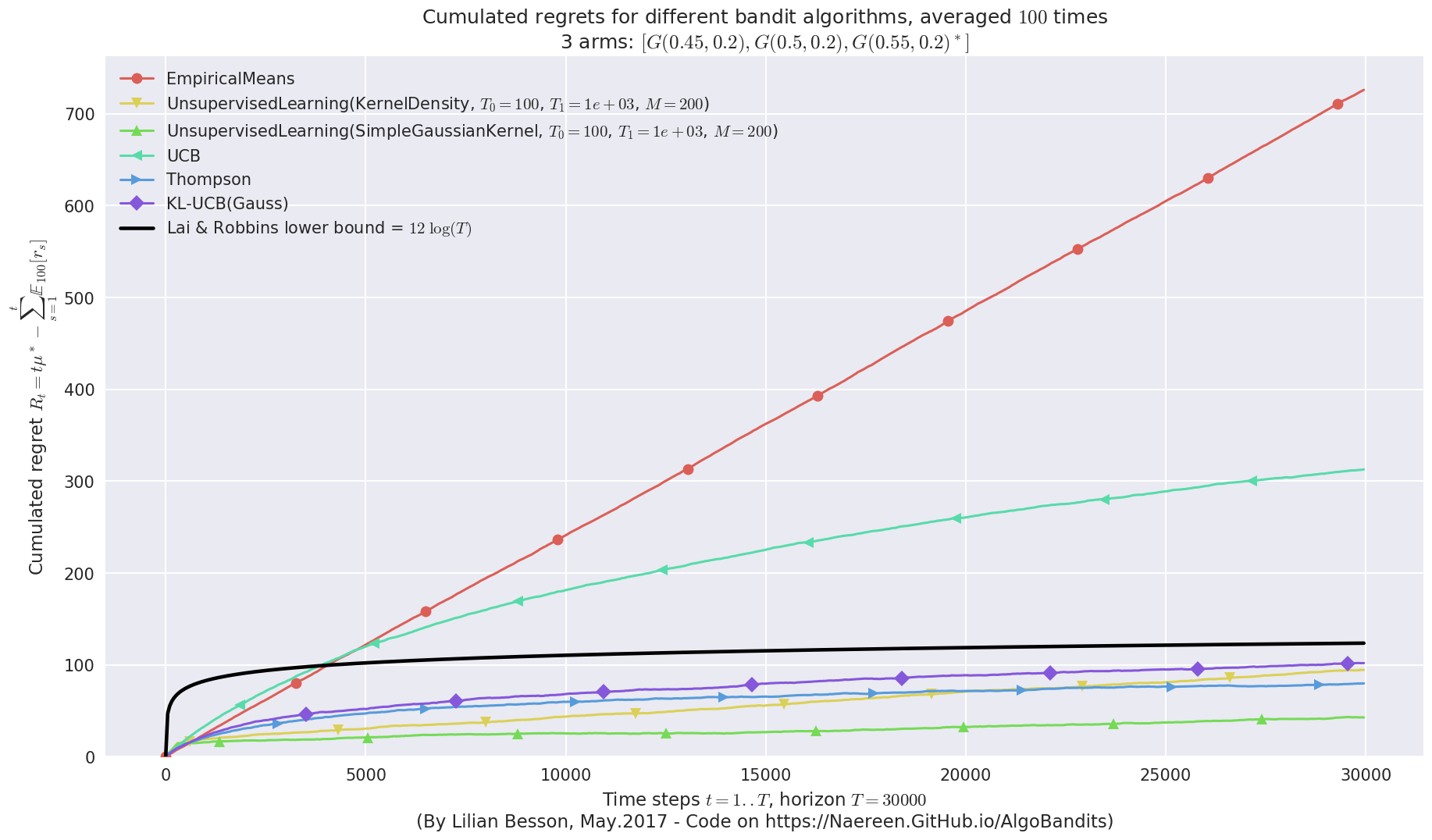
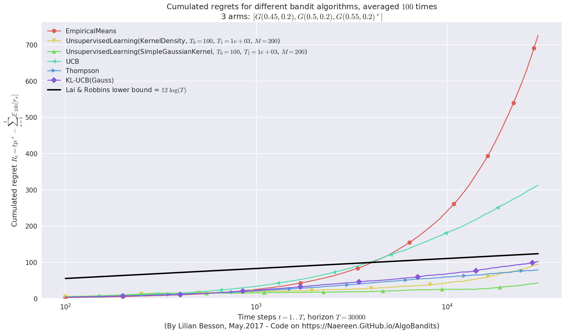
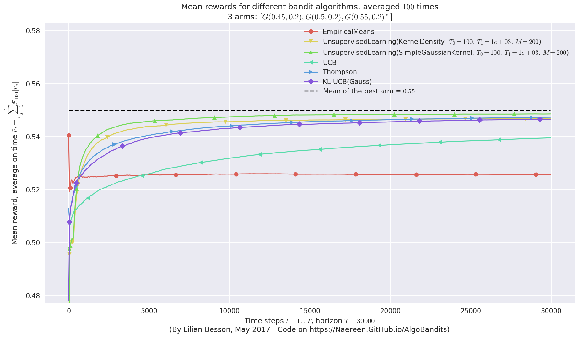
Now, we can plot some performance measures, like the regret, the best arm selection rate, the average reward etc.

def plotAll(evaluation, envId=0):
    evaluation.printFinalRanking(envId)
    evaluation.plotRegrets(envId)
    evaluation.plotRegrets(envId, semilogx=True)
    evaluation.plotRegrets(envId, meanRegret=True)
    evaluation.plotBestArmPulls(envId)

evaluation?

Type:        Evaluator
String form: <Environment.Evaluator.Evaluator object at 0x7f8357929978>
File:        ~/ownCloud/cloud.openmailbox.org/Thèse_2016-17/src/SMPyBandits.git/Environment/Evaluator.py
Docstring:   Evaluator class to run the simulations.

plotAll(evaluation)

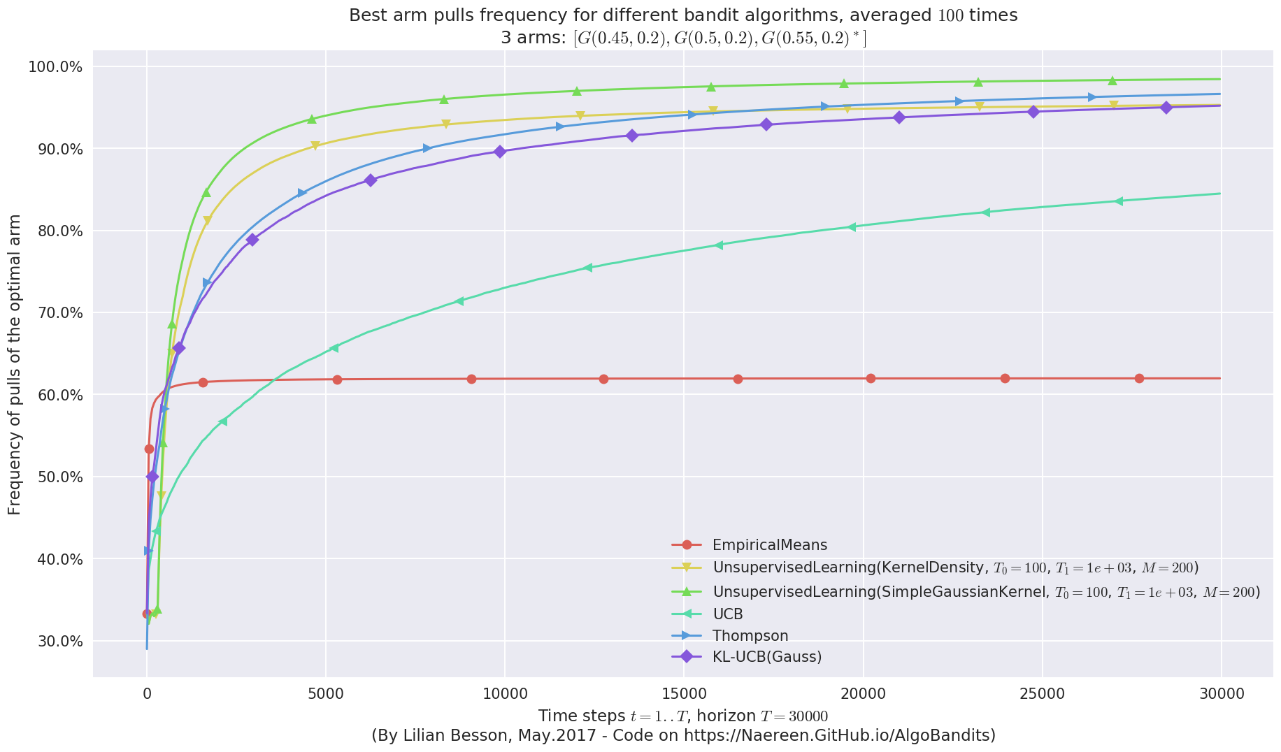
Final ranking for this environment #0 :
- Policy 'UnsupervisedLearning(SimpleGaussianKernel, $T_0=100$, $T_1=1e+03$, $M=200$)'  was ranked      1 / 6 for this simulation (last regret = 42.8587).
- Policy 'Thompson'     was ranked      2 / 6 for this simulation (last regret = 79.6796).
- Policy 'UnsupervisedLearning(KernelDensity, $T_0=100$, $T_1=1e+03$, $M=200$)' was ranked      3 / 6 for this simulation (last regret = 94.4365).
- Policy 'KL-UCB(Gauss)'        was ranked      4 / 6 for this simulation (last regret = 101.951).
- Policy 'UCB'  was ranked      5 / 6 for this simulation (last regret = 312.357).
- Policy 'EmpiricalMeans'       was ranked      6 / 6 for this simulation (last regret = 723.75).

This MAB problem has:
 - a [Lai & Robbins] complexity constant C(mu) = 12 for 1-player problem...
 - a Optimal Arm Identification factor H_OI(mu) = 61.67% ...

This MAB problem has:
 - a [Lai & Robbins] complexity constant C(mu) = 12 for 1-player problem...
 - a Optimal Arm Identification factor H_OI(mu) = 61.67% ...

This MAB problem has:
 - a [Lai & Robbins] complexity constant C(mu) = 12 for 1-player problem...
 - a Optimal Arm Identification factor H_OI(mu) = 61.67% ...

---

Another experiment, with just more Gaussian arms

HORIZON = 30000
REPETITIONS = 100
N_JOBS = min(REPETITIONS, 4)
means = [0.30, 0.35, 0.40, 0.45, 0.5, 0.55, 0.60, 0.65, 0.70]
ENVIRONMENTS = [ [Gaussian(mu, sigma=0.25) for mu in means] ]

POLICIES = [
        # --- Our algorithm, with two Unsupervised Learning algorithms
        {
            "archtype": UnsupervisedLearning,
            "params": {
                "estimator": KernelDensity,
                "kernel": 'gaussian',
                "bandwidth": sigma,
                "T_0": T_0,
                "fit_every": fit_every,
                "meanOf": meanOf,
            }
        },
        {
            "archtype": UnsupervisedLearning,
            "params": {
                "estimator": SimpleGaussianKernel,
                "T_0": T_0,
                "fit_every": fit_every,
                "meanOf": meanOf,
            }
        },
        # --- Basic UCB1 algorithm
        {
            "archtype": UCB,
            "params": {}
        },
        # --- Thompson sampling algorithm
        {
            "archtype": Thompson,
            "params": {}
        },
        # --- klUCB algorithm, with Gaussian klucb function
        {
            "archtype": klUCB,
            "params": {
                "klucb": klucb
            }
        },
    ]

configuration = {
    # --- Duration of the experiment
    "horizon": HORIZON,
    # --- Number of repetition of the experiment (to have an average)
    "repetitions": REPETITIONS,
    # --- Parameters for the use of joblib.Parallel
    "n_jobs": N_JOBS,    # = nb of CPU cores
    "verbosity": 6,      # Max joblib verbosity
    # --- Arms
    "environment": ENVIRONMENTS,
    # --- Algorithms
    "policies": POLICIES,
}

evaluation2 = Evaluator(configuration)

Number of policies in this comparison: 5
Time horizon: 30000
Number of repetitions: 100
Sampling rate for saving, delta_t_save: 1
Sampling rate for plotting, delta_t_plot: 50
Number of jobs for parallelization: 4
Creating a new MAB problem ...
  Taking arms of this MAB problem from a list of arms 'configuration' = [G(0.3, 0.25), G(0.35, 0.25), G(0.4, 0.25), G(0.45, 0.25), G(0.5, 0.25), G(0.55, 0.25), G(0.6, 0.25), G(0.65, 0.25), G(0.7, 0.25)] ...
 - with 'arms' = [G(0.3, 0.25), G(0.35, 0.25), G(0.4, 0.25), G(0.45, 0.25), G(0.5, 0.25), G(0.55, 0.25), G(0.6, 0.25), G(0.65, 0.25), G(0.7, 0.25)]
 - with 'means' = [ 0.3   0.35  0.4   0.45  0.5   0.55  0.6   0.65  0.7 ]
 - with 'nbArms' = 9
 - with 'maxArm' = 0.7
 - with 'minArm' = 0.3

This MAB problem has:
 - a [Lai & Robbins] complexity constant C(mu) = 27.2 ...
 - a Optimal Arm Identification factor H_OI(mu) = 68.89% ...
 - with 'arms' represented as: $[G(0.3, 0.25), G(0.35, 0.25), G(0.4, 0.25), G(0.45, 0.25), G(0.5, 0.25), G(0.55, 0.25), G(0.6, 0.25), G(0.65,$
$0.25), G(0.7, 0.25)^*]$
Number of environments to try: 1

Running the experiment

We asked to repeat the experiment \(100\) times, so it will take a while…

%%time
for envId, env in tqdm(enumerate(evaluation2.envs), desc="Problems"):
    # Evaluate just that env
    evaluation2.startOneEnv(envId, env)

Evaluating environment: MAB(nbArms: 9, arms: [G(0.3, 0.25), G(0.35, 0.25), G(0.4, 0.25), G(0.45, 0.25), G(0.5, 0.25), G(0.55, 0.25), G(0.6, 0.25), G(0.65, 0.25), G(0.7, 0.25)], minArm: 0.3, maxArm: 0.7)
- Adding policy #1 = {'archtype': <class '__main__.UnsupervisedLearning'>, 'params': {'bandwidth': 0.2, 'meanOf': 200, 'T_0': 100, 'kernel': 'gaussian', 'estimator': <class 'sklearn.neighbors.kde.KernelDensity'>, 'fit_every': 1000}} ...
  Creating this policy from a dictionnary 'self.cfg['policies'][0]' = {'archtype': <class '__main__.UnsupervisedLearning'>, 'params': {'bandwidth': 0.2, 'meanOf': 200, 'T_0': 100, 'kernel': 'gaussian', 'estimator': <class 'sklearn.neighbors.kde.KernelDensity'>, 'fit_every': 1000}} ...
- Adding policy #2 = {'archtype': <class '__main__.UnsupervisedLearning'>, 'params': {'estimator': <class '__main__.SimpleGaussianKernel'>, 'fit_every': 1000, 'meanOf': 200, 'T_0': 100}} ...
  Creating this policy from a dictionnary 'self.cfg['policies'][1]' = {'archtype': <class '__main__.UnsupervisedLearning'>, 'params': {'estimator': <class '__main__.SimpleGaussianKernel'>, 'fit_every': 1000, 'meanOf': 200, 'T_0': 100}} ...
- Adding policy #3 = {'archtype': <class 'Policies.UCB.UCB'>, 'params': {}} ...
  Creating this policy from a dictionnary 'self.cfg['policies'][2]' = {'archtype': <class 'Policies.UCB.UCB'>, 'params': {}} ...
- Adding policy #4 = {'archtype': <class 'Policies.Thompson.Thompson'>, 'params': {}} ...
  Creating this policy from a dictionnary 'self.cfg['policies'][3]' = {'archtype': <class 'Policies.Thompson.Thompson'>, 'params': {}} ...
- Adding policy #5 = {'archtype': <class 'Policies.klUCB.klUCB'>, 'params': {'klucb': <function klucbGauss at 0x7f835bfd9488>}} ...
  Creating this policy from a dictionnary 'self.cfg['policies'][4]' = {'archtype': <class 'Policies.klUCB.klUCB'>, 'params': {'klucb': <function klucbGauss at 0x7f835bfd9488>}} ...

- Evaluating policy #1/5: UnsupervisedLearning(KernelDensity, $T_0=100$, $T_1=1e+03$, $M=200$) ...

Estimated order by the policy UnsupervisedLearning(KernelDensity, $T_0=100$, $T_1=1e+03$, $M=200$) after 30000 steps: [0 1 2 3 4 5 6 7 8] ...
  ==> Optimal arm identification: 100.00% (relative success)...
  ==> Manhattan   distance from optimal ordering: 100.00% (relative success)...
  ==> Kendell Tau distance from optimal ordering: 99.98% (relative success)...
  ==> Spearman    distance from optimal ordering: 100.00% (relative success)...
  ==> Gestalt     distance from optimal ordering: 100.00% (relative success)...
  ==> Mean distance from optimal ordering: 100.00% (relative success)...

[Parallel(n_jobs=4)]: Done   5 tasks      | elapsed:   48.7s
[Parallel(n_jobs=4)]: Done  42 tasks      | elapsed:  4.3min

- Evaluating policy #2/5: UnsupervisedLearning(SimpleGaussianKernel, $T_0=100$, $T_1=1e+03$, $M=200$) ...

[Parallel(n_jobs=4)]: Done 100 out of 100 | elapsed:  9.8min finished

Estimated order by the policy UnsupervisedLearning(SimpleGaussianKernel, $T_0=100$, $T_1=1e+03$, $M=200$) after 30000 steps: [0 2 1 3 4 6 5 7 8] ...
  ==> Optimal arm identification: 100.00% (relative success)...
  ==> Manhattan   distance from optimal ordering: 90.12% (relative success)...
  ==> Kendell Tau distance from optimal ordering: 99.92% (relative success)...
  ==> Spearman    distance from optimal ordering: 100.00% (relative success)...
  ==> Gestalt     distance from optimal ordering: 77.78% (relative success)...
  ==> Mean distance from optimal ordering: 91.95% (relative success)...

[Parallel(n_jobs=4)]: Done   5 tasks      | elapsed:   19.8s
[Parallel(n_jobs=4)]: Done  42 tasks      | elapsed:  1.9min

- Evaluating policy #3/5: UCB ...

[Parallel(n_jobs=4)]: Done 100 out of 100 | elapsed: 477.2min finished

Estimated order by the policy UCB after 30000 steps: [0 2 6 5 4 1 7 3 8] ...
  ==> Optimal arm identification: 100.00% (relative success)...
  ==> Manhattan   distance from optimal ordering: 60.49% (relative success)...
  ==> Kendell Tau distance from optimal ordering: 85.56% (relative success)...
  ==> Spearman    distance from optimal ordering: 87.50% (relative success)...
  ==> Gestalt     distance from optimal ordering: 55.56% (relative success)...
  ==> Mean distance from optimal ordering: 72.28% (relative success)...

[Parallel(n_jobs=4)]: Done   5 tasks      | elapsed:    2.9s
[Parallel(n_jobs=4)]: Done  42 tasks      | elapsed:   16.1s
[Parallel(n_jobs=4)]: Done 100 out of 100 | elapsed:   38.7s finished

- Evaluating policy #4/5: Thompson ...

Estimated order by the policy Thompson after 30000 steps: [2 0 4 3 1 5 6 7 8] ...
  ==> Optimal arm identification: 100.00% (relative success)...
  ==> Manhattan   distance from optimal ordering: 80.25% (relative success)...
  ==> Kendell Tau distance from optimal ordering: 99.33% (relative success)...
  ==> Spearman    distance from optimal ordering: 99.63% (relative success)...
  ==> Gestalt     distance from optimal ordering: 66.67% (relative success)...
  ==> Mean distance from optimal ordering: 86.47% (relative success)...

[Parallel(n_jobs=4)]: Done   5 tasks      | elapsed:    4.1s
[Parallel(n_jobs=4)]: Done  42 tasks      | elapsed:   22.4s
[Parallel(n_jobs=4)]: Done 100 out of 100 | elapsed:   52.8s finished

- Evaluating policy #5/5: KL-UCB(Gauss) ...

Estimated order by the policy KL-UCB(Gauss) after 30000 steps: [0 2 3 1 5 7 6 4 8] ...
  ==> Optimal arm identification: 100.00% (relative success)...
  ==> Manhattan   distance from optimal ordering: 75.31% (relative success)...
  ==> Kendell Tau distance from optimal ordering: 98.77% (relative success)...
  ==> Spearman    distance from optimal ordering: 99.47% (relative success)...
  ==> Gestalt     distance from optimal ordering: 66.67% (relative success)...
  ==> Mean distance from optimal ordering: 85.05% (relative success)...

[Parallel(n_jobs=4)]: Done   5 tasks      | elapsed:    7.2s
[Parallel(n_jobs=4)]: Done  42 tasks      | elapsed:   40.4s

CPU times: user 2.56 s, sys: 656 ms, total: 3.22 s
Wall time: 8h 10min 4s

[Parallel(n_jobs=4)]: Done 100 out of 100 | elapsed:  1.6min finished

Visualizing the results

Now, we can plot some performance measures, like the regret, the best arm selection rate, the average reward etc.

plotAll(evaluation2)

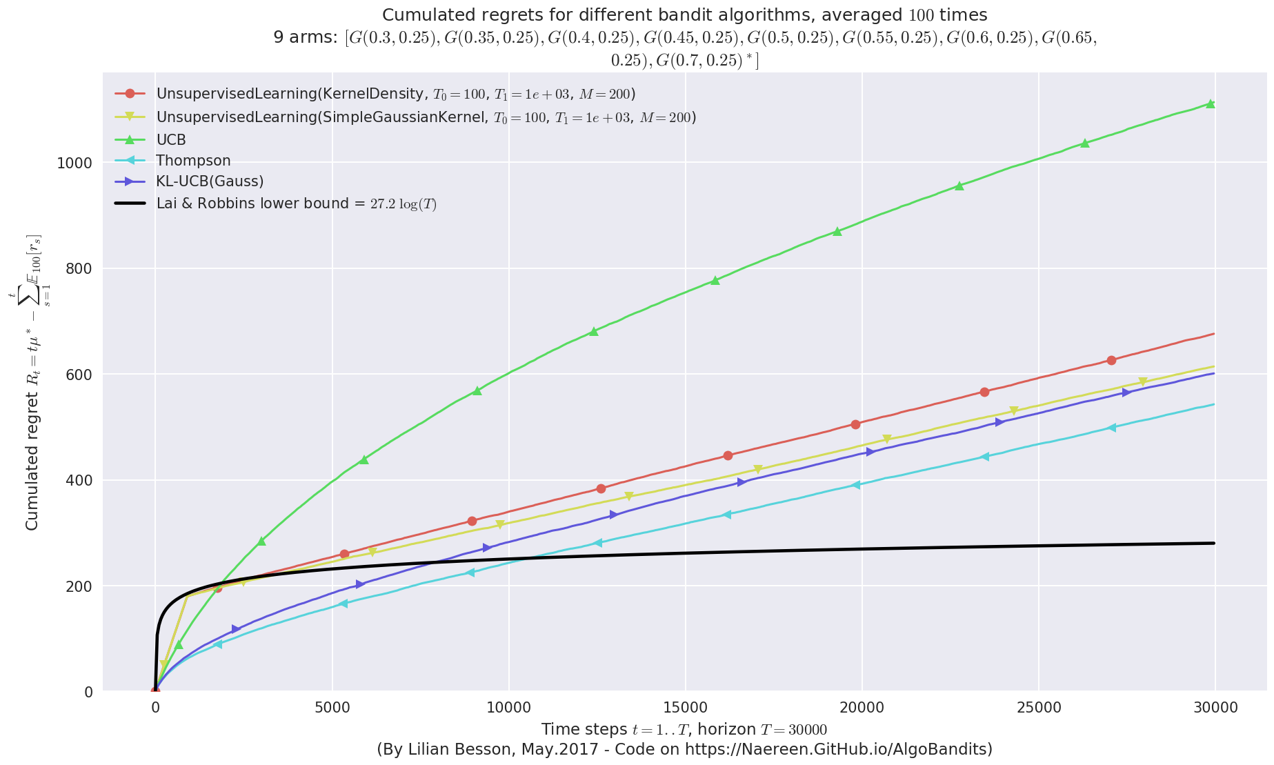
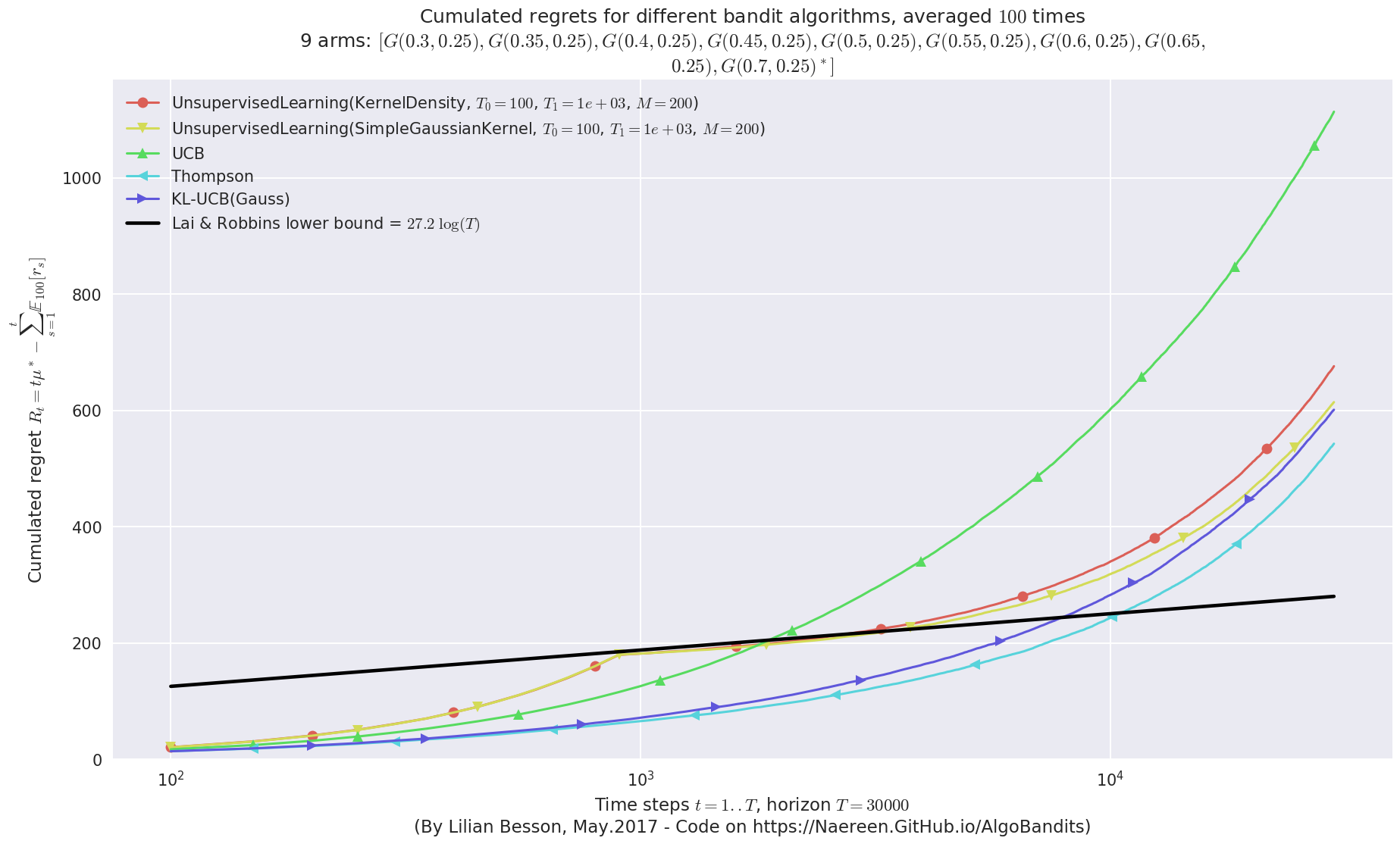
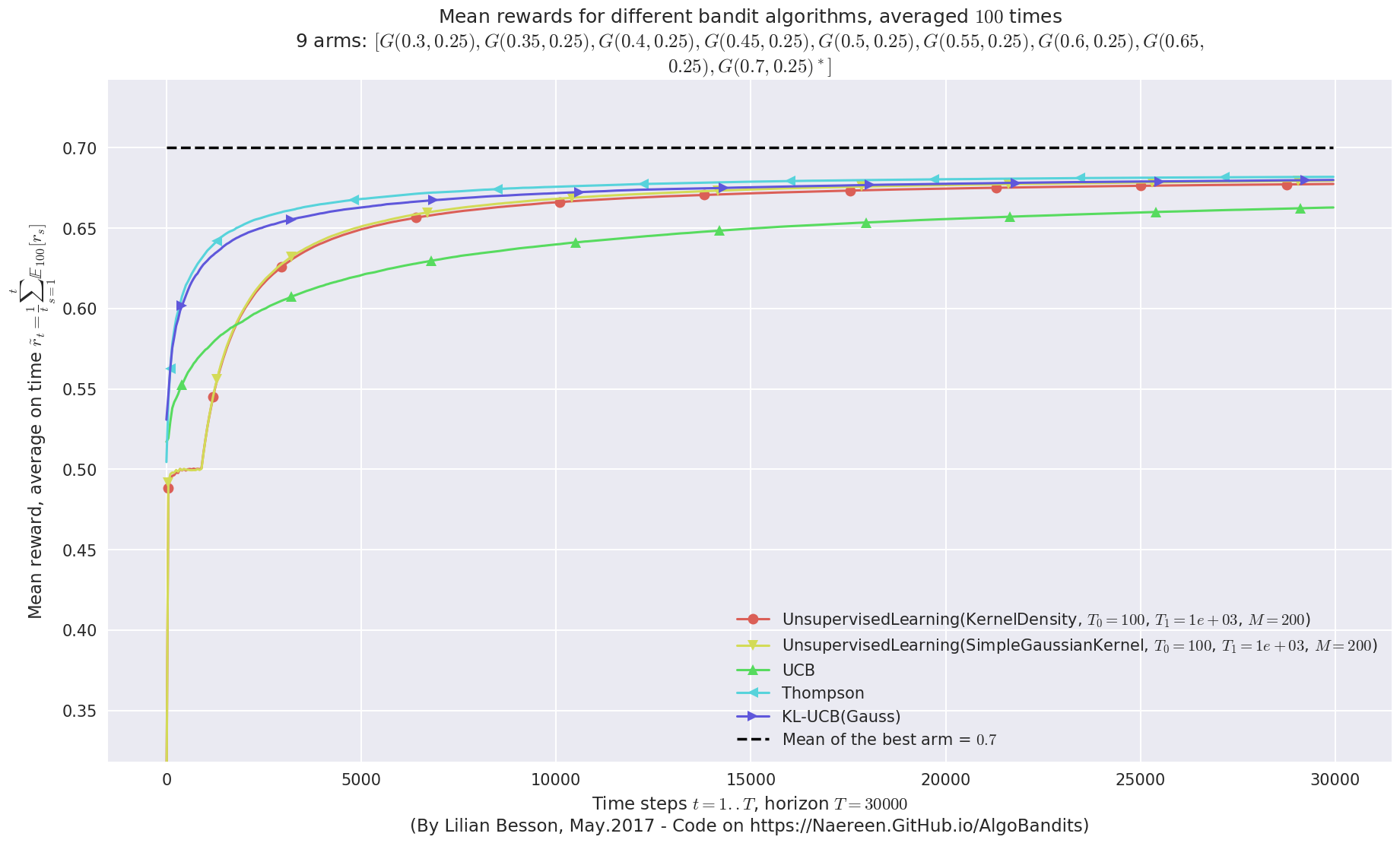
Final ranking for this environment #0 :
- Policy 'Thompson'     was ranked      1 / 5 for this simulation (last regret = 541.01).
- Policy 'KL-UCB(Gauss)'        was ranked      2 / 5 for this simulation (last regret = 599.75).
- Policy 'UnsupervisedLearning(SimpleGaussianKernel, $T_0=100$, $T_1=1e+03$, $M=200$)'  was ranked      3 / 5 for this simulation (last regret = 612.761).
- Policy 'UnsupervisedLearning(KernelDensity, $T_0=100$, $T_1=1e+03$, $M=200$)' was ranked      4 / 5 for this simulation (last regret = 674.086).
- Policy 'UCB'  was ranked      5 / 5 for this simulation (last regret = 1111.22).

This MAB problem has:
 - a [Lai & Robbins] complexity constant C(mu) = 27.2 for 1-player problem...
 - a Optimal Arm Identification factor H_OI(mu) = 68.89% ...

This MAB problem has:
 - a [Lai & Robbins] complexity constant C(mu) = 27.2 for 1-player problem...
 - a Optimal Arm Identification factor H_OI(mu) = 68.89% ...

This MAB problem has:
 - a [Lai & Robbins] complexity constant C(mu) = 27.2 for 1-player problem...
 - a Optimal Arm Identification factor H_OI(mu) = 68.89% ...

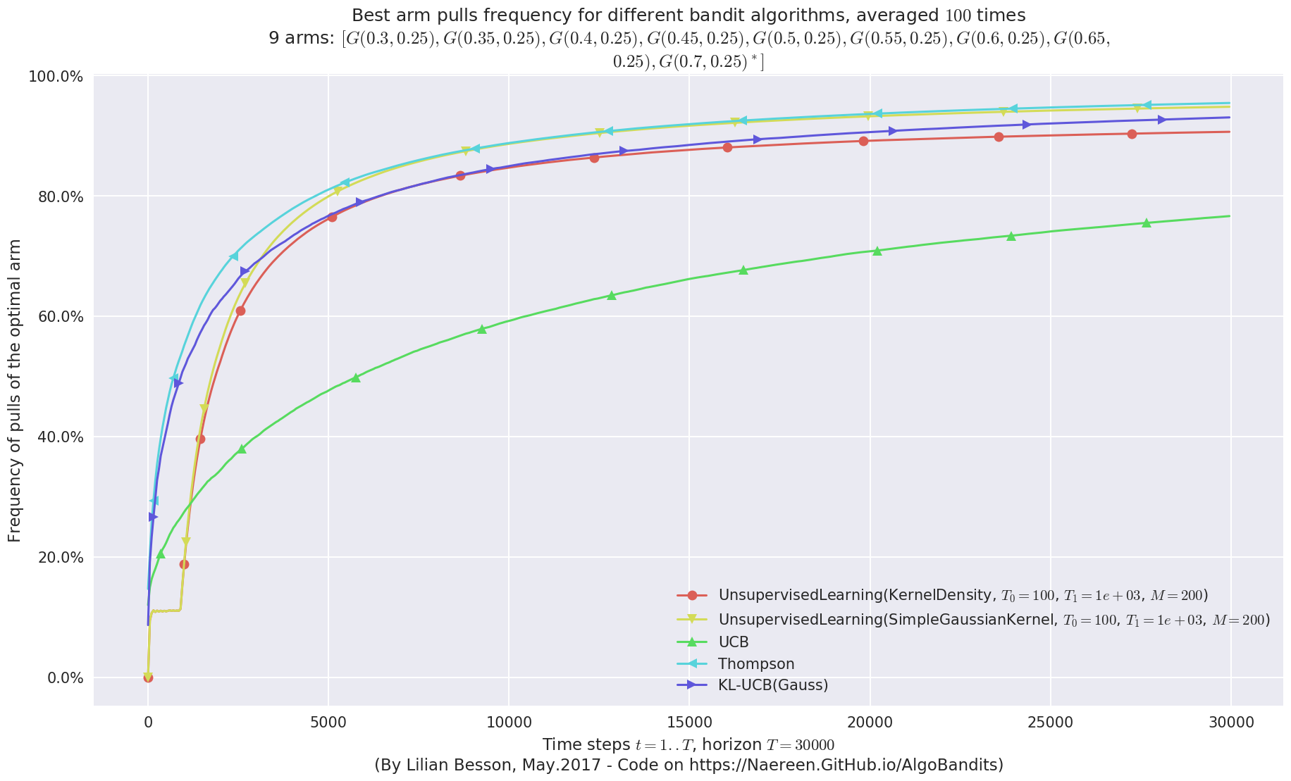
Very good performance!

Whoo, on this last experiment, the simple UnsupervisedLearning(SimpleGaussianKernel) works as well as Thompson Sampling (Thompson) !!

… In fact, it was almost obvious : Thompson Sampling uses a Gamma posterior, while UnsupervisedLearning(SimpleGaussianKernel) works very similarly to Thompson Sampling (start with a flat kernel, fit it to the data, and to take decision, sample it and play the arm with the highest sample). UnsupervisedLearning(SimpleGaussianKernel) basically uses a Gaussian posterior, which is obviously better than a Gamma posterior for Gaussian arms!

---

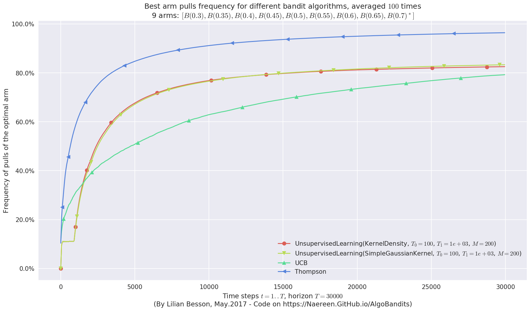
Another experiment, with Bernoulli arms

Let also try the same algorithms but on Bernoulli arms.

from Arms import Bernoulli

HORIZON = 30000
REPETITIONS = 100
N_JOBS = min(REPETITIONS, 4)
means = [0.30, 0.35, 0.40, 0.45, 0.5, 0.55, 0.60, 0.65, 0.70]
ENVIRONMENTS = [ [Bernoulli(mu) for mu in means] ]

POLICIES = [
        # --- Our algorithm, with two Unsupervised Learning algorithms
        {
            "archtype": UnsupervisedLearning,
            "params": {
                "estimator": KernelDensity,
                "kernel": 'gaussian',
                "bandwidth": 0.1,
                "T_0": T_0,
                "fit_every": fit_every,
                "meanOf": meanOf,
            }
        },
        {
            "archtype": UnsupervisedLearning,
            "params": {
                "estimator": SimpleGaussianKernel,
                "T_0": T_0,
                "fit_every": fit_every,
                "meanOf": meanOf,
            }
        },
        # --- Basic UCB1 algorithm
        {
            "archtype": UCB,
            "params": {}
        },
        # --- Thompson sampling algorithm
        {
            "archtype": Thompson,
            "params": {}
        },
    ]

configuration = {
    # --- Duration of the experiment
    "horizon": HORIZON,
    # --- Number of repetition of the experiment (to have an average)
    "repetitions": REPETITIONS,
    # --- Parameters for the use of joblib.Parallel
    "n_jobs": N_JOBS,    # = nb of CPU cores
    "verbosity": 6,      # Max joblib verbosity
    # --- Arms
    "environment": ENVIRONMENTS,
    # --- Algorithms
    "policies": POLICIES,
}

evaluation3 = Evaluator(configuration)

Number of policies in this comparison: 4
Time horizon: 30000
Number of repetitions: 100
Sampling rate for saving, delta_t_save: 1
Sampling rate for plotting, delta_t_plot: 50
Number of jobs for parallelization: 4
Creating a new MAB problem ...
  Taking arms of this MAB problem from a list of arms 'configuration' = [B(0.3), B(0.35), B(0.4), B(0.45), B(0.5), B(0.55), B(0.6), B(0.65), B(0.7)] ...
 - with 'arms' = [B(0.3), B(0.35), B(0.4), B(0.45), B(0.5), B(0.55), B(0.6), B(0.65), B(0.7)]
 - with 'means' = [ 0.3   0.35  0.4   0.45  0.5   0.55  0.6   0.65  0.7 ]
 - with 'nbArms' = 9
 - with 'maxArm' = 0.7
 - with 'minArm' = 0.3

This MAB problem has:
 - a [Lai & Robbins] complexity constant C(mu) = 24.3 ...
 - a Optimal Arm Identification factor H_OI(mu) = 68.89% ...
 - with 'arms' represented as: $[B(0.3), B(0.35), B(0.4), B(0.45), B(0.5), B(0.55), B(0.6), B(0.65), B(0.7)^*]$
Number of environments to try: 1

Running the experiment

We asked to repeat the experiment \(100\) times, so it will take a while…

%%time
for envId, env in tqdm(enumerate(evaluation3.envs), desc="Problems"):
    # Evaluate just that env
    evaluation3.startOneEnv(envId, env)

Evaluating environment: MAB(nbArms: 9, arms: [B(0.3), B(0.35), B(0.4), B(0.45), B(0.5), B(0.55), B(0.6), B(0.65), B(0.7)], minArm: 0.3, maxArm: 0.7)
- Adding policy #1 = {'archtype': <class '__main__.UnsupervisedLearning'>, 'params': {'bandwidth': 0.1, 'meanOf': 200, 'T_0': 100, 'kernel': 'gaussian', 'estimator': <class 'sklearn.neighbors.kde.KernelDensity'>, 'fit_every': 1000}} ...
  Creating this policy from a dictionnary 'self.cfg['policies'][0]' = {'archtype': <class '__main__.UnsupervisedLearning'>, 'params': {'bandwidth': 0.1, 'meanOf': 200, 'T_0': 100, 'kernel': 'gaussian', 'estimator': <class 'sklearn.neighbors.kde.KernelDensity'>, 'fit_every': 1000}} ...
- Adding policy #2 = {'archtype': <class '__main__.UnsupervisedLearning'>, 'params': {'estimator': <class '__main__.SimpleGaussianKernel'>, 'fit_every': 1000, 'meanOf': 200, 'T_0': 100}} ...
  Creating this policy from a dictionnary 'self.cfg['policies'][1]' = {'archtype': <class '__main__.UnsupervisedLearning'>, 'params': {'estimator': <class '__main__.SimpleGaussianKernel'>, 'fit_every': 1000, 'meanOf': 200, 'T_0': 100}} ...
- Adding policy #3 = {'archtype': <class 'Policies.UCB.UCB'>, 'params': {}} ...
  Creating this policy from a dictionnary 'self.cfg['policies'][2]' = {'archtype': <class 'Policies.UCB.UCB'>, 'params': {}} ...
- Adding policy #4 = {'archtype': <class 'Policies.Thompson.Thompson'>, 'params': {}} ...
  Creating this policy from a dictionnary 'self.cfg['policies'][3]' = {'archtype': <class 'Policies.Thompson.Thompson'>, 'params': {}} ...

- Evaluating policy #1/4: UnsupervisedLearning(KernelDensity, $T_0=100$, $T_1=1e+03$, $M=200$) ...

Estimated order by the policy UnsupervisedLearning(KernelDensity, $T_0=100$, $T_1=1e+03$, $M=200$) after 30000 steps: [0 2 1 3 4 5 6 7 8] ...
  ==> Optimal arm identification: 100.00% (relative success)...
  ==> Manhattan   distance from optimal ordering: 95.06% (relative success)...
  ==> Kendell Tau distance from optimal ordering: 99.96% (relative success)...
  ==> Spearman    distance from optimal ordering: 100.00% (relative success)...
  ==> Gestalt     distance from optimal ordering: 88.89% (relative success)...
  ==> Mean distance from optimal ordering: 95.98% (relative success)...

[Parallel(n_jobs=4)]: Done   5 tasks      | elapsed:   59.6s
[Parallel(n_jobs=4)]: Done  42 tasks      | elapsed:  5.4min

- Evaluating policy #2/4: UnsupervisedLearning(SimpleGaussianKernel, $T_0=100$, $T_1=1e+03$, $M=200$) ...

[Parallel(n_jobs=4)]: Done 100 out of 100 | elapsed: 12.4min finished

Estimated order by the policy UnsupervisedLearning(SimpleGaussianKernel, $T_0=100$, $T_1=1e+03$, $M=200$) after 30000 steps: [0 2 3 1 4 5 6 7 8] ...  ==> Kendell Tau distance from optimal ordering: 99.92% (relative success)...

  ==> Optimal arm identification: 100.00% (relative success)...
  ==> Manhattan   distance from optimal ordering: 90.12% (relative success)...
  ==> Spearman    distance from optimal ordering: 99.99% (relative success)...
  ==> Gestalt     distance from optimal ordering: 88.89% (relative success)...
  ==> Mean distance from optimal ordering: 94.73% (relative success)...

[Parallel(n_jobs=4)]: Done   5 tasks      | elapsed:   20.4s
[Parallel(n_jobs=4)]: Done  42 tasks      | elapsed:  2.0min

- Evaluating policy #3/4: UCB ...

[Parallel(n_jobs=4)]: Done 100 out of 100 | elapsed:  4.6min finished

Estimated order by the policy UCB after 30000 steps: [0 4 2 3 1 6 5 7 8] ...
  ==> Optimal arm identification: 100.00% (relative success)...
  ==> Manhattan   distance from optimal ordering: 80.25% (relative success)...
  ==> Kendell Tau distance from optimal ordering: 98.77% (relative success)...
  ==> Spearman    distance from optimal ordering: 99.47% (relative success)...
  ==> Gestalt     distance from optimal ordering: 66.67% (relative success)...
  ==> Mean distance from optimal ordering: 86.29% (relative success)...

[Parallel(n_jobs=4)]: Done   5 tasks      | elapsed:    2.7s
[Parallel(n_jobs=4)]: Done  42 tasks      | elapsed:   15.6s
[Parallel(n_jobs=4)]: Done 100 out of 100 | elapsed:   35.9s finished

- Evaluating policy #4/4: Thompson ...

Estimated order by the policy Thompson after 30000 steps: [2 4 0 3 1 5 6 7 8] ...
  ==> Optimal arm identification: 100.00% (relative success)...
  ==> Manhattan   distance from optimal ordering: 75.31% (relative success)...
  ==> Kendell Tau distance from optimal ordering: 98.77% (relative success)...
  ==> Spearman    distance from optimal ordering: 98.75% (relative success)...
  ==> Gestalt     distance from optimal ordering: 66.67% (relative success)...
  ==> Mean distance from optimal ordering: 84.87% (relative success)...

[Parallel(n_jobs=4)]: Done   5 tasks      | elapsed:    3.5s
[Parallel(n_jobs=4)]: Done  42 tasks      | elapsed:   20.3s
[Parallel(n_jobs=4)]: Done 100 out of 100 | elapsed:   48.7s finished

CPU times: user 2.21 s, sys: 584 ms, total: 2.79 s
Wall time: 18min 25s

Visualizing the results

Now, we can plot some performance measures, like the regret, the best arm selection rate, the average reward etc.

plotAll(evaluation3)

Final ranking for this environment #0 :
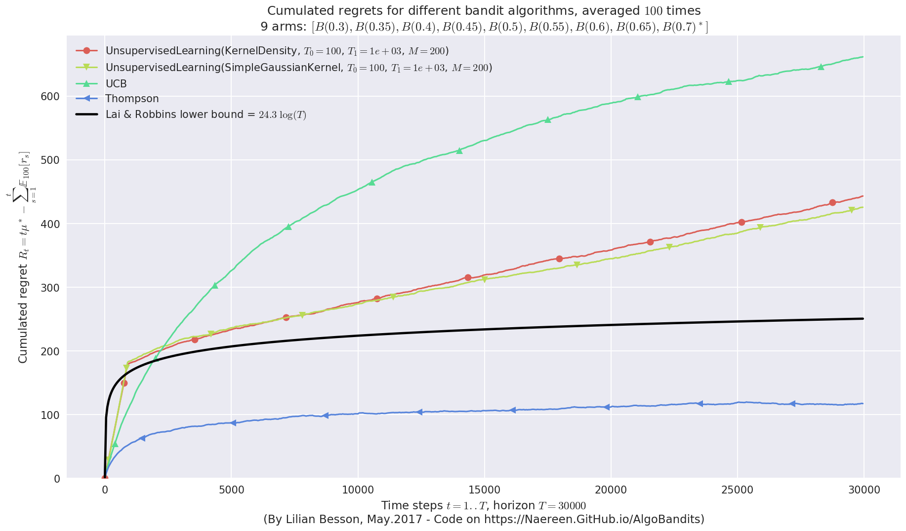
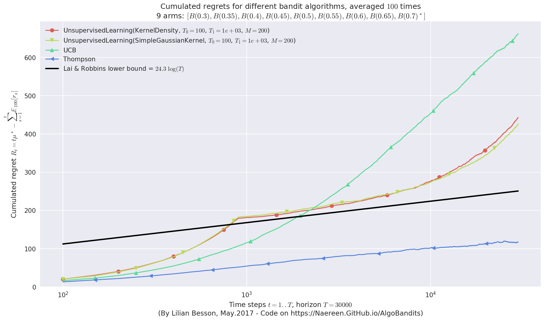
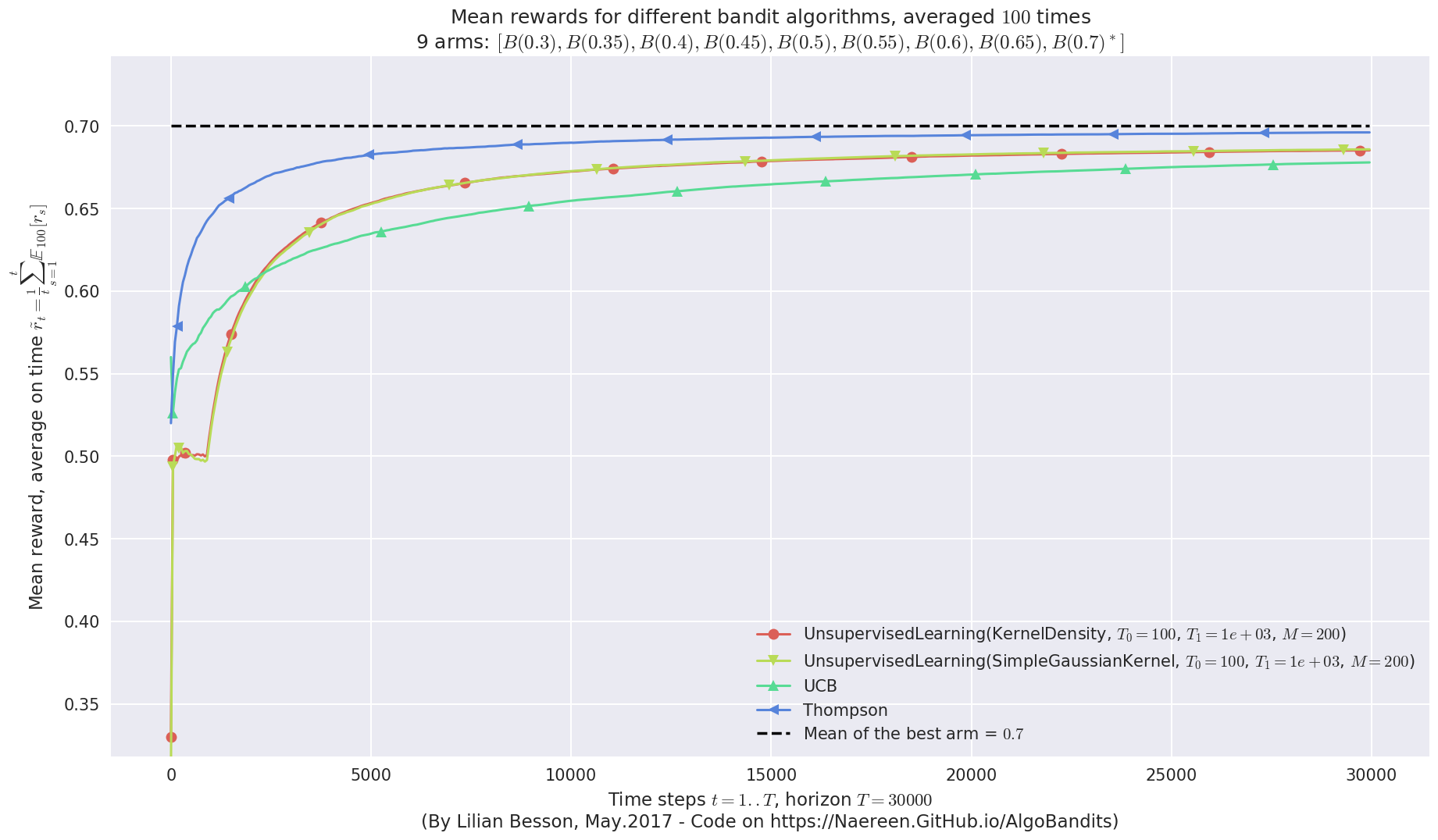
- Policy 'Thompson'     was ranked      1 / 4 for this simulation (last regret = 117.25).
- Policy 'UnsupervisedLearning(SimpleGaussianKernel, $T_0=100$, $T_1=1e+03$, $M=200$)'  was ranked      2 / 4 for this simulation (last regret = 425.23).
- Policy 'UnsupervisedLearning(KernelDensity, $T_0=100$, $T_1=1e+03$, $M=200$)' was ranked      3 / 4 for this simulation (last regret = 441.91).
- Policy 'UCB'  was ranked      4 / 4 for this simulation (last regret = 661.27).

This MAB problem has:
 - a [Lai & Robbins] complexity constant C(mu) = 24.3 for 1-player problem...
 - a Optimal Arm Identification factor H_OI(mu) = 68.89% ...

This MAB problem has:
 - a [Lai & Robbins] complexity constant C(mu) = 24.3 for 1-player problem...
 - a Optimal Arm Identification factor H_OI(mu) = 68.89% ...

This MAB problem has:
 - a [Lai & Robbins] complexity constant C(mu) = 24.3 for 1-player problem...
 - a Optimal Arm Identification factor H_OI(mu) = 68.89% ...

---

Conclusion

This small simulation shows that with the appropriate tweaking of parameters, and on reasonably easy Gaussian Multi-Armed Bandit problems, one can use a Unsupervised Learning learning algorithm, being a non on-line algorithm (i.e., updating it at time step \(t\) has a time complexity about \(\mathcal{O}(K t)\) instead of \(\mathcal{O}(K)\)).

By tweaking cleverly the algorithm, mainly without refitting the model at every steps (e.g., but once every \(T_1 = 1000\) steps), it works as well as the best-possible algorithm, here we compared against Thompson (Thompson Sampling) and klUCB (kl-UCB with Gaussian \(\mathrm{KL}(x,y)\) function).

When comparing in terms of mean rewards, accumulated rewards, best-arm selection, and regret (loss against the best fixed-arm policy), this UnsupervisedLearning(KernelDensity, ...) algorithm performs as well as the others.

Non-logarithmic regret

But in terms of regret, it seems that the profile for UnsupervisedLearning(KernelDensity, ...) is not asymptotically logarithmic, contrarily to Thompson and klUCB (cf. see the first curve above, at the end on the right).

• Note that the horizon is not that large, \(T = 30000\) is not very long.
• And note that the four parameters, \(T_0, T_1, M\) for the UnsupervisedLearning part, and \(\mathrm{bandwidth}\) for the KernelDensity part, have all been (manually) tweaked for this setting. For instance, \(\mathrm{bandwidth} = \sigma = 0.2\) is the same as the one used for the arms (but in a real-world scenario, this would be unknown), \(T_0,T_1\) is adapted to \(T\), and \(M\) is adapted to \(\sigma\) also (to reduce variance of the samples for the models).

Comparing time complexity

Another aspect is the time complexity of the UnsupervisedLearning(KernelDensity, ...) algorithm. In the simulation above, we saw that it took about \(42\;\mathrm{min}\) to do \(1000\) experiments of horizon \(T = 30000\) (about \(8.4 10^{-5} \; \mathrm{s}\) by time step), against \(5.5\;\mathrm{min}\) for Thompson Sampling : even with fitting the unsupervised learning model only once every :math:`T_1 = 1000` steps, it is still about \(8\) times slower than Thompson Sampling or UCB !

It is not that much, but still…

time_by_loop_UL_KD = (42 * 60.) / (REPETITIONS * HORIZON)
time_by_loop_UL_KD

0.00084

time_by_loop_TS = (5.5 * 60.) / (REPETITIONS * HORIZON)
time_by_loop_TS

0.00011

42 / 5.5

7.636363636363637

Not so efficient for Bernoulli arms

Similarly, the last experiment showed that this UnsupervisedLearning policy was not so efficient on Bernoulli problems, with a Gaussian kernel.

A better approach could have been to use a Bernoulli “kernel”, i.e., fitting a Bernoulli distribution on each arm.

I implemented this for my framework, see here the documentation for ``SimpleBernoulliKernel` <https://smpybandits.github.io/docs/Policies.UnsupervisedLearning.html#Policies.UnsupervisedLearning.SimpleBernoulliKernel>`__, but I will not present it here.

---

This notebook is here to illustrate my SMPyBandits library, for which a complete documentation is available, here at https://smpybandits.github.io/.

That’s it for this demo! See you, folks!